Quadrilateral finite element for thin and thick plates

Plates are the basic components for various modern engineering structures. Constructing the plate finite element model, we necessary consider that plates can have the various thicknesses. The finite element method is widely used to calculate the plates. It is very important that the plate finite element can be using to calculate, with equal success, the thin and thick plates. Many finite elements were constructed by now, but researchers are still being conducted to obtain other elements. An important research area is the development of models for accounting the shear deformations of thick plates.

In paper [1] the quadrilateral four node plate element, in which each node contains seven degrees of freedom, is considered. The plate kinematics are described using a third-order shear deformation plate theory, without the need for special treatment of shear-locking effect and shear correction factors. The accuracy of the proposed approach assessed on numerical results is confirmed by comparing the obtained results with respect to reference published solutions. Weak form Galerkin’s method is used for the development of the finite element model in article [2]. In this study is developed locking-free rectangular finite elements for shear deformable 2-D Mindlin, Levinson and Full Interior plates. In each the finite element node there is three degrees of freedom. The paper [3] presents a new simple four-node quadrilateral shell element with 24-dof which can be used to analyze thick and thin shell problems. This element which is developed from DKMQ plate element using the Naghdi/Mindlin/Reissner shell theory can consider warping effects and coupling bending-membrane energy. The incomplete quadratic interpolation functions are used for approximations of rotations. In article [4] is presented the method for incorporating shear flexibility into existing three-node triangular thin plate elements with particular relevance to finite element templates. In the paper noted that the method is not restricted to finite element templates and is independent of the thin plate formulation, but not all thin plate elements are suitable candidates for use as the parent elements of shear deformable elements. The authors of the paper [5] proposed two finite element methods for solving the Reissner-Mindlin plate problem. The problem is solved either by augmenting the Galerkin’s formulation or modifying the plate-thickness. In these methods, the transverse displacement is approximated by conforming (bi)linear macro elements or (bi)quadratic elements, and the rotation by conforming (bi)linear elements.

An important and developing area of research is analyses of functionally graded material isotropic and sandwich plates with considering the shear deformations [6]–[8]. In study [6] a weak Galerkin’s form was used to discretize the governing partial differential equations that are numerically solved by NURBS basic functions. Besides using polynomial function, any functions varying through the plate thickness can be used in this formulation if those functions are satisfied with the free conditions of shear stresses. Several examples with different geometries, stiffness ratios and boundary conditions were illustrated. The study [9] presents nonlinear bending analyses of functionally graded carbon nanotube-reinforced composite plates using the modified mesh-free radial point interpolation method.

For the reduction of shear-locking, in article [10] used modified formulation of Mindlin's plate theory. In this formulation, the shear strains are incorporated as degrees of freedom in lieu of the rotational in the conventional Mindlin's theory formulation. The natural element method using the concept of hierarchical models of plate-like elastic structures was presented in [11]. The displacement field in the thickness direction was assumed by 1-D polynomials, while the in-plane displacement field on the midsurface was numerically approximated. The numerical experiments were performed to illustrate the proposed method and to investigate the characteristics of hierarchical models. The paper [12] deals with the formulation of the cell centered finite volume application for plate bending analysis based on Mindlin– Reissner plate theory. In this formulation shape functions are used to represent the variation of the unknown variables across the control volumes’ faces, which facilitates the calculation of stress resultants on the faces. In paper noted that although the method behaves well in the test problems involving thin plates, however further studies are needed to investigate whether the method is shear locking-free in the thin plate analysis. In study [13] the discrete Kirchhoff–Mindlin theory is applied to arbitrary polygons using the transverse displacements and the rotations. The transverse shear effect is included by assuming that the tangential shear strain is constant along each edge of the polygon. The shear locking phenomenon is then alleviated by relating the kinematical and the independent shear strain along each edge of the polygon. The authors of the article [14] offer to use the modified Mindlin theory and to split total deflection and two slope angles of plate cross–sections into their constitutive parts, resulting with decomposition of plate state on flexure and transverse shear. The paper [15] is devoted to improving the theory of bending and vibrations of three-layer plates with transverse compressible filler and thin outer bearing layers. The equations of the bi-moment theory of thick plates with respect to forces, moments and bi-moments, created in the framework of the three-dimensional theory of elasticity, taking into account the nonlinearity of the distribution law of displacements and stresses over the thickness, are taken as the equations of motion of the filler. In the article [16] is presented calculations of composite plates, considering the finite stiffness of the seams and the nonlinear behavior of the materials of the layers by the iteration method and the sequential solution of linear equations. The alternative solution for the plate calculation with assuming shear deformations was presented in the articles [17]. The solution has been based on piecewise constant approximations of the moments and shear forces. Using the virtual displacements principle, the algebraic equilibrium equations was constructed independently for bend and shear states. The equilibrium equations with using Lagrange’s multipliers added into the additional energy functional. The similar approach is using in [18] for a plane elasticity problem, in [1921] for a bending plate analysis.

The proposed paper aim is to construct the quadrilateral finite element based on linear approximations of moments for calculations thin and thick plates.

2    Materials and Methods

For calculation, a bending plate considering the shear deformations we shall use the additional energy functional for an isotropic plate (for simplicity, we assume there are no specified displacements):

n c =¹ 12 (m ² + M 2² -2 vMM + M ²)dA+¹ Nll L ) (q² + Q^dA.         (1)

• _{2 Et} 3 x y        x y xy        _{2 Et}        x y

E is the material elasticity modulus; t is the plate thickness; v is Poisson's ratio; k = 6/5 is the coefficient resulting from the parabolic law of tangential stress changing across the plate thickness. The functional (1) is can written in matrix form that is more convenient if we use a finite element method:

П c =¹ S T E ^-1 S dA.

In expression (2) the following notation is entered:

S T = ( M x M y M xy Q x Q y ) .

In accordance with the principle of the additional energy minimum, the moments M_x M_y M_xy and shear forces Q_x Q_y must satisfy the corresponding differential equilibrium equations (4) and static boundary conditions.

dM 8M„      8MV 8M       dQ Q

---x +--- xy - Q_x = 0,---^ +--- xy - Q = 0, -Q x +   + q = 0.

d x     d y           d y     d x    ^y      d x    d y

Dividing the problem region into finite elements and using the moments and forces approximations, then we replace the differential equations (7) by algebraic equations system. For this we shall use the weighted residuals method. Then for the first differential equation, we can write the following equations of the weighted residuals method:

Jv

A i ^k

(d M   d M

---x +---xy

dx     d y

^^^^H

Q x 50 _x3 dA = 0, i = 1,2, ... N .

N is the nodes number of the finite element grid; 50_x i is the weight function of node /; A i is the area where the weight function is nonzero. We shall use the node weight functions which are nonzero only in the finite element’s region adjacent to it. Such weight functions can be called “local”. Using for (5) the integration procedure in parts, we obtain the following expression:

J M

а ( ее_хД

A i

к

dx

d ( 50_xl )          d ( M_x50_xl )   d ( M 0 Y

M„ V xi’ + Qx50x, + v ^ ^’i7 + v ^ x,lJ dA = 0, i = 1,2,_N. xy                       x x ,i dy              dx         dy

The two last terms in expression (6) can be transformed using the Gauss theorem [1] (integration by parts in the plane case) into the integral over the region boundary, then we get:

г      d ( 50_i )

[ m ^{v x,i)} + M

J ^x     dx         xy

A . к

а ( 5в х,' )

d y

^^^^™

Q_x50_x, dA - f ( M_xl_x + M_x l \80_x dr = 0, i = 1,2, _ N . x x , i                     x x xy y      x , i

r

ri is the area boundary where the weight function 50xi is nonzero; lx,l are direction cosines of the region ri boundary normal; Ai is the area of the finite elements which adjacent to node /. The expression (7) coincides with the term of possible displacements principle if we use the rotation angle along the X axis as the possible displacement. Also, the expression (7) let us to consider the static boundary conditions for the moments Mx , Mxy . The first integral in (7) is the work of the internal moments and forces at possible displacements, the second integral is the external moments potential, which act on the boundary.

Performing similar transformations to the second and third equations (7), we obtain equilibrium equations sets:

two more

_r(     a ( 50„ )       0 ( 50,, )         )      _f,_     _ _

J M y YY+ M» YY- Q y ⁵⁰ yi dA-- J ( M y i y + M x*¹- K^{d r=} 0 i= ^1>2- N•

A к       °y                           7       ^r i

( d (5w) d (5w f Qx Ay2+Qy -yy2

A k      ^{d x          d} y 7

dA - J ( Q x l x + Q , l , ) 5 wjdr - J q 5 w i dA = 0, i = 1,2, _ N .

r i

A i

50yi is the possible rotation angle along the axis Y (weight function); 5wi is the possible vertical displacement (weight function); Qx , Qy are the external forces on the boundary. If there are not the moments and forces distributed along the free boundary then second integrals in (7–9) are zero.

We get algebraic equilibrium equations system (7–9) which are the limitations of the functional (2).

The algebraic equilibrium equations system can be presented in the matrix form (10):

Tyukalov Yu.

Quadrilateral finite element for thin and thick plates;

L S S - P = 0.                                          (10)

These limitations can be included to functional by using the Lagrange's multipliers w (11):

n c = 2 J S T E - 1 S dA+ w ^T ( L S S - P ) .                              (11)

The matrix L _S lines number equal the number of all node equilibrium equations. The vector P elements are defined by external loads which act to the plate.

Note, the internal moments and forces derivatives are not come in expressions (2), (7–9), so any functions can be taken for the moments and forces approximations. The equilibrium equations include only the possible displacements first derivatives, so the possible displacements can be the linear functions.

We use for the moment approximation in a finite element region the following linear functions (12):

M x = a ₁ + a ₂ x + a ₃ y, M y = b ₁ + b ₂ x + b ₃ y , M_xy = c ₁ + c ₂ x + c ₃ y .                   (12)

a ₁, a ₂, a ₃, b ₁, b ₂, b ₃, c ₁, c ₂, c ₃ are unknown parameters of the approximations’ functions. Using the equations (4) we get the expressions of the shear forces (13):

Q x = ^a 2 ^{+ c} 3 , ^Qy = b 3 ^{+ c} 2 "                                        ⁽¹³⁾

So, if there is no distributed load in a finite element area, the differential equations (4) are in progress. We introduce the following vectors for the finite element k (14):

S ^T = ( ^M x   ^My  ^Mxy  ^Qx  ^Qy ) , a ^T = ( a l   ^a 2   ^a 3   b l   b 2   ^b 3   c l   ^c 2   ^C 3 ) •            (14)

Then we can write the expressions (12) and (13) in matrix form (15, 16): 1   x  y  0  0  0  0  0  0 0  0  0  1   x  y  0  0  0 S k = Ga k , G = 0  0  0  0  0  0  1   x  y • 0  1   0  0  0  0  0  0  1 0  0  0  0  0  1   0  1   0 The specific flexibility matrix of the material has the following form: [ '2  -^    0       0       0  1 Et 3     E 3 "- 1 V  21    0      0      0 Et 3      Et 3 Ek =   0     0     24(1 +V )     0        0 k                          Et 3 0     0      0      1 21+ V )     0 5 Et 12(1 +v) 0       0         0           0          ( v )

(15) .                            (16)

_ "       "         "           "          5 Et . Using (14) – (16), we get the following expression of the functional (2) for th n k = 1 J a T ( G T E t G ) a k dA. 2 A k The flexibility matrix of a finite element is (18): D k = J G T E k G dA. Ak

e finite element k (17): (17) (18)

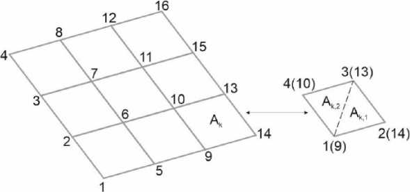
Fig. 1 - Dividing the finite element area by the two triangles

For defining the matrix Dk elements it is necessary to calculate the following integrals by the finite element area (19):

i x = J x ^dA, i y = J y dA, i xx = J ^X 2 ^dA, i xy = J xy dA i yy = J У 2 dA.

Ak              Ak               Ak                Ak                Ak

If we divide the finite element on two triangles (Fig. 1), then these integrals are simple calculated analytically using the triangle coordinates system. Use (19) we get the matrix D _k elements expressions

(20):

	F d i A k           d i i x           d i i y	d 2 A k	d 2 ix	d 2 iy	0	0	0       "
	d 4 Ak + d i i xx      d i i xy	di 2 x	di xx	d 2 ixy	0	0	d 4 A k
	d 1 iyy	d 2 iy	d 2 ixy	d 2 iyy	0	0	0
		d 1 A k	d 1 ix	d 1 iy	0	0	0
D k =			d 1 ixx	d 1 ixy	0	0	0	.            (20)
	symmetrically			d 4 A k + d i i yy	0	d 4 A k	0
					d 4 A k	d 3 ix	d 3 iy
						d 4 A k + d 3 i xx	d 3 ixy
	[						d 4 A k + d 3 i yy _
In (21) it had been introduced designations:
d = 12- d =				2 ( i + v ) d i,		i2 ( i + v ) .		(21)
		-V d i ,	d 3 =		d 4 =
1 Et 3     2						5 Et

From matrix Dk it is constructed the matrix D of whole plate. Number columns and rows of matrix is 9 ■ Ne. Ne is number of finite elements. Matrix D have the block diagonal form and it is easy converted (22):

D 1

D =

D 2

D

Ne

We also use linear functions for approximations of possible displacements in finite element area (Fig. 2):

^ w i = ^a i,i + ^a 2i x + ^а з дУ + ^a 4,i xy , ⁵⁹ xi = « li + ^a 2,i x + ^а 3 дУ + « 4 , i Xy , 59 _y i = a _i i + a ₂ ix + a ₃ iy + a 4 i xy ,    i = 1,2,3 ,4.

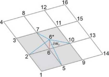
Fig. 2 - Possible displacement of a node

To calculate the parameters a ji we form the following matrix:

	1 X 1    У 1    X 1 У 1
	1 x 2 У 2 x 2 У 2
B =		.                                             (24)
	1   x 3    У з    x 3 У з
	- 1 x 4    У 4   x 4 У 4 _

If the possible displacement of node is taken equal to unity, then the parameters a_{j , i} are elements of the inverse matrix B ^-1 (25):

a11    a1,2    a1,3    a1,4 B-1 = a2,1   a2,2 a2,3 a2,4 -                                            (25) a3,1   a3,2   a3,3   a3,4 _a4,1   a4,2   a4,3   a4,4 _ Each column of the matrix B-1 contains the approximating functions parameters for possible displacement of one finite element node. Each column of the matrix B-1 contains the approximating functions parameters for possible displacement of one finite element node.

Now we shall calculate the equilibrium equation (7) when there is the node i possible rotation 56x i along axis X. The derivatives of the rotation angle will have these expressions (26):

а^Д я а^Д

5kx = —4—- = a i+a,у , 5k„ = —4—- = a,+a xx                           2 i 4 i         xy                           3 i 4 i ox                      оу

The internal forces possible work 5U^₆ of the finite element k will get next form (7):

• ^5U^ 6_X = J ( a l ⁺ a 2^{X +} a 3 У ) ( « 2i ^{+ a} 4 ,- У ) ^{dA +} J ( ^C 1 ⁺ c 2 ^{X +} c 3 У ) ( « 3,i ^{+ a} 4i x ) ^dA

A k                                                 A k

• - ( a. + c ) f a ,. + a X + a у + a ,xy) dA.

• 2       3         1 i 2 i 3 i 4 i

A k

Another we can say that 5и^ ₆ is contribution of finite element to equilibrium equation (7). For calculation of the integrals, we use the expressions (19). Then we get follow matrix term (28):

	' a 2iAk + a 4i i y ' - a i,i A k — a 3i i y a 2i i y + « 4Ay
	0
5 U 0 = C ^ ak , C;A =.	0
	0
	a 3,i A k + a 4i i x a 3i i x + a 4i i xx - а 1 , iAk — « 2, i i x

For the possible rotation 50_yi we similarly get (8):

^{5 U}U 9 _y = J ( ^b 1 + ^b 2 x + ^Ь 3 у ) ( « 3,i + « 4,i x ) ^dA + J ( c l + c 2 x + c 3 У ) ( « 2,i + « 4 ,1У ) ^dA

A k                                                A k

- J ( ^b 3 + c 2 ) ( « 1, i + « 2,i x + « 3,iy + « 4, X ) ^dA

A k

	0
	0
	0
	a 3iAk + a 4,i i x
5U 0 = C T S y a k , C i e y =•	« 3,i i x + « 4,i i xx -aV i A k — « 2Л a 2iAk + a 4J i y - aViA k — « 3i i y _ a 2i i y + a 4, i i yy

At the vertical possible displacement 5 w i finite element shear forces do the possible work (9):
5 Uiw = J ( a 2 + c3 ) ( a 2, i + «^ y ) dA	+ J ( b 3 + c2 ) ( a	3, i + a 4,i x ) dA-                       (31)
Ak	Ak
	0
	a 2, A + a 4,i i y
	0
	0
5 U *, = C Tw a k . C w =J	0	[•                                       (32)
	« 3, A + a 4,i i x
	0
	a 3,iAk + a 4,i i x
	a2A + a 4J i y

Using (28), (30), (32) it can be constructed the matrix "equilibrium" of the finite element:

T = Г                                                                                    1

Each matrix Lk line is the contribution of the finite element to the node equilibrium equation on corresponding possible displacement. From matrix Lk , in accordance with nodes and finite elements numbering, it is formed the global equilibrium matrix L of whole plate.

The last integral in (9) is the external loads potential which caused by possible displacement 5w i .

If q is uniformly distributed load this integral for the finite element k is calculated analytically:

J q ⁵ w i dA = q («^Д + « . i x + а_{з д}i y + « 4^ i xy ) = P k -

Ak

With accordance node numbering the value Pk, is added to the element of global vector P . Moreover, the concentrated at the nodes forces values Pz, must be added to the elements of global vector P .

Now the functional (11) can be written in the next form (35):

П ^с = - a ^T Da + w ^T ( La - P ) .

The vector Lagrange’s multipliers w are included the values of the node’s vertical displacements and rotation angles, which are free. Calculating the functional derivatives along the vectors a and w we get the matrix equations system:

Da + L ^T w = 0, La + P = 0.

Expressing the vector a from the first equation and substituting it into the second equation, we obtain:

K = LD ^-1 L ^T , Kw = P , a = - D ^-1 L ^T w .                               (37)

Expressions (12), (13) allow us to get the moments and forces values for any finite element point. But, as rules, these values are calculated for finite element center. The global matrix K also can be get as sum of the local matrices K _k of finite elements:

K k = L k D - ¹ L - ¹ .                                        (38)

This algorithm is the same as one of classical finite element method based on displacements approximations.

3    Results and Discussion3.1    Levi's plates

To verify the accuracy of the present finite element it had been calculated the rectangular plates with various boundary conditions (Fig. 3). It was calculated the plates with different values of the aspect ratio b / a and the thickness-to-side ratio t / a .

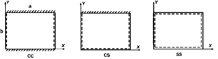
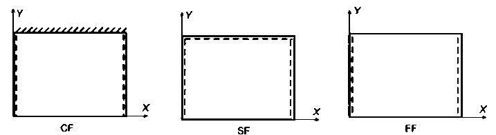
Fig. 3 - The support variants of the Levi's plates

In Fig. 3 dashed lines and the letter S denotes simply supported sides, the oblique hatching and the letter C denotes clamped sides, and the letter F denotes free sides. Data: a = 3; E = 1000; v = 0.3; q = 10 .Boundary conditions: w = 6 x = 6_y = 0 for side denote C; w = 0 and 0_{x ( y} ) = 0 ( ^ x ( _y ) is rotation angle along boundary side) for S; w = 0 for F. Table 1 presents the calculations results of these plates, given in [22] for two theories, and the results obtained by the proposed method which is denoted MAP. The lengths of the plate sides are equal 3 or 1.5. The side 3 long was divided into 30 finite elements, and the side 1.5 long into 16 elements. The load is evenly distributed over the plate area. The calculations results are presented in Tables and Figures in dimensionless form:

w =

100Et ³ (a b A 1 (a b A 777, 2\ 4 ^w I T’E? I^,M x = 2M x I "^’T" I^, 12 ( 1 -v ² ) qa 72 2 ) qa к2 2 )

1       (a b A 1       (a , A

My =   2" My I       I, My-s =   2" My I 7', b I • qa    к 2 2)       qa     к 2 )

The S-FSDT is simple first-order shear deformation theory in which the vertical displacement is separated into a bending and shear parts. The TV-FSDT is two variable first-order shear deformation theory presented in [22]. In that paper, there is used an analytical method for the calculation Levi’s plates. Analyzing the results given in Table 1, we must note, the decisions of the MAP method are very close to the TV-FSDT decisions for all plate thickness values and the boundary conditions. For all considering plate variants, the plate center displacement values calculated by the MAP method, are larger the values calculated the other methods. For the CC plate with parameters t / a = 0.001, a I b = 2 was received the biggest difference of the results. It is about 10 percenters. If the ratio 1 1 a increase, then the results difference become lower. For the plates with other parameters the results difference does not exceed 3 percenters. In general, we note the proposal methods MAP can be used for calculations the thin and thick plates and the known locking effect for thin plates is absent.

Table 1. Displacement of the plate center w under the uniformly distributed load action

a/b	t/a	Method	Boundary conditions
			CC	CS	SS	CF	SF	FF
2	0.001	S-FSDT	0.0163	0.0305	0.0633	0.1450	0.3809	1.3713
		TV-FSDT	0.0163	0.0305	0.0633	0.1450	0.3810	1.3714
		MAP	0.0163	0.0305	0.0634	0.1461	0.3833	1.3701
	0.04	S-FSDT	0.0176	0.0318	0.0646	0.1476	0.3835	1.3770
		TV-FSDT	0.0178	0.0322	0.0646	0.1504	0.3879	1.3795
		MAP	0.0178	0.0322	0.0648	0.1510	0.3892	1.3775
	0.1	S-FSDT	0.0245	0.0386	0.0714	0.1614	0.3972	1.4070
		TV-FSDT	0.0255	0.0407	0.0714	0.1721	0.4084	1.4130
		MAP	0.0255	0.0407	0.0716	0.1726	0.4096	1.4108
	0.2	S-FSDT	0.0489	0.0630	0.0958	0.2105	0.4464	1.5142
		TV-FSDT	0.0525	0.0695	0.0958	0.2395	0.4692	1.5248
		MAP	0.0526	0.0697	0.0961	0.2401	0.4706	1.5225
1	0.001	S-FSDT	0.1917	0.2786	0.4062	0.5667	0.7931	1.3094
		TV-FSDT	0.1917	0.2786	0.4062	0.5667	0.7931	1.3094
		MAP	0.1924	0.2795	0.4075	0.5676	0.7937	1.3076
	0.04	S-FSDT	0.1951	0.2819	0.4096	0.5712	0.7975	1.3151
		TV-FSDT	0.1965	0.2830	0.4096	0.5737	0.7981	1.3154
		MAP	0.1972	0.2841	0.4111	0.5743	0.7988	1.3135
	0.1	S-FSDT	0.2128	0.2996	0.4273	0.5945	0.8208	1.3451
		TV-FSDT	0.2209	0.3059	0.4273	0.6065	0.8224	1.3459
		MAP	0.2216	0.3070	0.4290	0.6071	0.8231	1.3440
	0.2	S-FSDT	0.2759	0.3827	0.4904	0.6777	0.9041	1.4522
		TV-FSDT	0.3021	0.3827	0.4904	0.7139	0.9072	1.4539

		MAP	0.3031	0.3841	0.4923	0.7145	0.9081	1.4519
0.5	0.001	S-FSDT	0.8445	0.9270	1.0129	1.0605	1.1496	1.2887
		TV-FSDT	0.8445	0.9270	1.0129	1.0605	1.1496	1.2887
		MAP	0.8484	0.9301	1.0150	1.0600	1.1479	1.2831
	0.04	S-FSDT	0.8497	0.9322	1.0181	1.0660	1.1551	1.2944
		TV-FSDT	0.8511	0.9330	1.0181	1.0664	1.1547	1.2938
		MAP -	0.8550	0.9362	1.0205	1.0661	1.1534	1.2885
	0.1	S-FSDT	0.8770	0.9596	1.0454	1.0946	1.1837	1.3244
		TV-FSDT	0.8850	0.9637	1.0454	1.0981	1.1829	1.3228
		MAP	0.8888	0.9671	1.0483	1.0978	1.1819	1.3176
	0.2	S-FSDT	0.9746	1.0572	1.1430	1.1970	1.2861	1.4316
		TV-FSDT	1.0000	1.0704	1.1430	1.2090	1.2844	1.4283
		MAP	1.0038	1.0741	1.1464	1.2087	1.2836	1.4231

3.2    Distorted grid for square plate with hinge supports under uniform loading Fig. 4 - Distorted grid 8 x 8 for one quarter of square plate

To analyze sensitive to finite element form distortion we calculated the square plate with the series distorted grids. The example of the distorted grid for one quarter of the plate is shown in Fig. 4. Due to symmetry, we will calculate only one quarter of the plate with hinge supports under uniform loading. The results are presented in Table 2. The designations MAP are the solutions obtained with square grids. Data: L = 12; t = 0.2,1,2.4; E = 10; v = 0.3; q = 1. Boundary conditions: w = Ox = 0 along sides AB and w = Oy = 0 along sides AD. Symmetry conditions: Ox = 0 along sides BC and Oy = 0 along sides CD.