Quantile metrics of risk assessment

• 1    Introduction to Value at Risk

“VaR is a monetary estimation of a variable (in basic currency) which will not be exceeded by expected losses during a given time span with a given probability.” [4,63]

“VaR are losses of a portfolio of assets which are not to be exceeded during a given time span with a given probability.” [6,47]

VaR is essentially a risk indicator, demonstrating a maximum loss, expressed in cash, for an investment portfolio/ instrument during a given time span, with a given confident probability level (confidence interval). This indicator allows to quantify potential portfolio expenses in monetary terms under normal market behavior. In other words, VaR method is not very efficient during economic crisis.

With a steady portfolio of positions (both long and short positions, reflected in the assets) and a given confidence level (1 – α) , confidence interval h , VaR is defined as a value (expressed in portfolio measurement units) which cover all possible portfolio losses during the time span h with probability (1 – α) .

P(X≤VaR)=1-α (5)

Considering the above mentioned formula, VaR is the biggest losses value being a consequence of assets returns instability.

The calculation reflects data which takes the following into account:

• -    Pre-determined time horizon h

• -    Significance level α (or confidence level 1 – α)

• -    Distribution assumptions

Holding period is a period which essentially depends on the portfolio instrument’s liquidity. As a rule, a time span sufficient to realize an asset so that the value won’t become negative (to close a position).

Confidence level is a probability indicator, chosen according to relationship to risks. In particular sector (as in banking) this variable is pre-defined to constitute 99% which is deemed optimal, but some other probabilities are used: 95% in Risk Metric or 99.7% in ratings firms’ approaches.

There are various approaches to interpreting VaR estimation. Let’s give an example of interpreting this indicator for the portfolio of 1 million RUR, time horizon of 1 day and a confidence level of 99%:

• -    Probability that the portfolio owner loses less than 1 million RUR within next 24 hours is 99%

• -    Probability that the losses of the portfolio owner will exceed 1 million RUR within next 24 hours is 1%

• -    Probability of expected losses exceeding 1 million RUR per portfolio equals to 1/100, which is once in a hundred days.

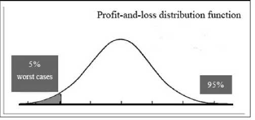
The curve depicted in Figure 3 illustrates normal distribution (though we can think of other kinds of distribution as well), which is composed by distribution of portfolio returns in a particular time interval.

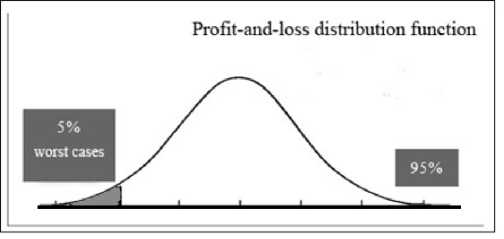
Grapf 3. Determining the value of VaR on the diagram of profit-and-loss distribution

The area of the diagram which is not painted represents 95% of the total shape’s area and a confidence level of 95% (or the significance level of 5%). VaR is a maximum amount of potential losses for the confidence level illustrated in the Figure.

In the case of f_∆P (x) being a returns probabilities distribution function, there can be the following interconnection between VaR and the confidence interval established:

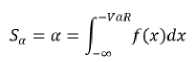
And, represented graphically – Figure 15:

Where S_α=α is a highlighted area representing 5% of the worst cases in Fig. 3

Estimation of VaR may be carried out in an absolute and relative sense. If VaR is relative, the estimation is made in

Grapf 4. Absolute and relative estimation of VaR

relation to the zero value. In case of relative estimation, the average returns level is added to the absolute value.

Furthermore, there are two approaches toVaR estimation:

• -    Approach which is based on local valuation where a linear or more complex approximation of instrument value function is being used

• -    Approach which is based on full valuation, where instrument’s value is recalculated and no approximations are employed.

VaR methods are used for:

• -    Estimation of returns for instruments/operations, taking risk indicators into account

• -    Implementing reasonable limits policy and limits computation on open positions

• -    Calculating/measuring capital sufficiency, as well as its placements in different businesses.

Thus, we can distinguish a number of advantages pertaining to VaR methodology, which enable us to assess metrics’ performance:

• -    Equals to the sum which can be lost with more or less probability;

• -    Gauges risk or risk factors on the basis of their sensitivity;

• -    Can be subject to comparison on particular markets;

• -    This is a generic method of measurement, applicable to all assets and types of risk;

• -    Can be measured on any level, be it an individual instrument level or a portfolio level;

• -    When risk aggregation or risk segmentation is used, there is an opportunity for improved study of assets interdependencies within a portfolio.

• 2. Market risk estimation models with VaR. Covariance method of computing VaR value

Variance-covariance method, also referred to as parametric, analytical or delta-normal method of VaR computing, assumes that all primary assets’ prices are normally distributed, therefore shaping value of the whole portfolio.

For assets returns computations (rt), logarithmical increment of prices are generally used rt= lnPt /Pt-1 = ln(Pt) – ln(P(t-1)) ~ N(µ, σ2)        (7)

Nevertheless, other methods for returns’ computations, covered in Chapter 1, can be equally implied.

Taking the formula for continuous accrual of interest as a basis, we can come up with the following equation:

An assumption on normal distribution of risk’s portfolio factors greatly facilitates the process of obtaining VaR value, because instruments’ returns distribution, enclosed in the given portfolio, will also be normal. This feature remains true for any instrument with linear characteristics of the price (currencies, shares).

In case of a random variable’s distribution, corresponding to normal type, the confidence interval ( 1 – α ) is characterized only by a quantile ( k_1–α ), which demonstrates random variable’s target position in relation to an average ( r ) shown among volatilities of the given portfolio ( σ_t ).

Having an investment position, comprising one instrument, we obtain the asset’s profit/loss in the amount of its daily value change. Thus, the smallest expected price with a probability (1 – α) can be formulated as follows:

P(t+1,1+α) = Pt exp(μi-k1-α σi)(9)

where P_t denotes the current price

Which can also be shown as,

P(t+1,1+α) =Pt eμ_i-k-1-α σ_i

Mathematical expectation of returns (one-day returns) is often taken as zero [4,212] which yields

P(t+1,1+α) =Pt e-k_(1-α) σ_i

VaR(1-α) =P(t+1)-Pt = Pt e-k_(1-α) σ_i -Pt(12)

(e│-k1-α σi-1)VaR(1-α) = Pt(13)

When computing VaR, in most cases we use linear approximation of value (e│-k_1-α σ_i-1) , which during Taylor expansion roughly equals ( -k_(1-α) σ_i ) when working with small variables¹. Also the negative sign of the value is often omitted, leading thus to the creation of a relative value.

VaR_(1-α) =-k_(1-α) σ_i,                         (14)

where σ_i denotes volatility, k_1-α is a quantile corresponding to the confidence interval (1 - α).

N-day value for VaR can be computed using the following equation:

N - day = VaR_1-day*√NVaR₁             (15)

However such an estimation is applicable for relatively short time spans only (10-15 days), and in cases of increasing time frames, the risk of inaccurate calculated data will find itself in direct dependence with the scaling interval.

Delta-normal method has the following advantages:

• -     Simple estimation method implementation

• -     High speed of computations

• -    Possible use of different indicators of volatility and correlation.

Drawbacks of the delta-normal method:

• -    Inability to obtain efficient data for distributions, other than normal, for the reason of heavy tails of distribution

• -    Inability to account nonlinear instruments’ risks accurately

• -    Complexity for understanding by top management

Probability of significant mistakes in used models.