"Information visualization” was first appeared in "The Cognitive Co-processor for Interactive User Interfaces" [1] published by Robertson, Card and Mackinlay. After that articles and researches about information visualization Start to appear, information visualization as a discipline has grown up. Information visualization combines with interactive, digital image processing, graphics and other disciplines, and it is a visual interface between person and information.

When air pollutants emitted in the air, it will be mixed with air forming mist. Mist is a common and complex natural phenomena, and different concentrations of mist effects on the ambience we will get different results. Mist as a participatory medium in image rendering remains a real challenge, but that image processing method plays a very important role in air pollutants visualization.

With the continuous development of industry, air pollution control and environment monitoring have attracted much attention from not only the governments

Manuscript received by ICIECS September 26, 2010; revised October 3, 2010; accepted October 8, 2010.

but also researchers. Nowadays, 2D display of scientific data can no longer satisfy the increasing requirement on realistic and immersive observation of large-scale data sets. With great development in graphics processing units, rendering scientific data in 3D has become more and more popular. It’s well-known that data visualization in 3D is much more complex than 2D, especially when the input data sets are large-scale. Therefore, real-time rendering of large-scale data has been one of the research focuses in scientific data visualization.

In this paper, we propose a novel real-time rendering algorithm to visualize large-scale air pollution data in 3D based on image processing. Given the density of air pollutants about some discrete places in the city, we first map the density values to different gray levels. Since the original data has some problems, the distribution of gray level undesirable. So we do spatial domain image enhancement processing on the gray levels to make them reasonable[2], and then construct a smooth surface according the discrete density (gray level) to represent the continuous density change in real world through B-spline [3][4][5]. Given view points and required resolution, we resample the constructed smooth surface to obtain gray levels of those air pollutants visible from current view point. Then we integrate the gray levels into each pixel of background [6] [7], and we can get a better result of reflecting the change of density in detail.

In the next section, we introduce the related work of data visualization and image processing. In section 3 we describe the original data model and data processing method. Section 4 introduces the novel method of B-spline surface interpolation which we used to construct the density surface. Finally the rendering method and the results are shown in section 5 before the conclusion in section 6.

• II.    Related work

Two areas of previous work are important to this paper: cloud rendering and fog rendering. Existing work for realistic fog and cloud rendering can be broadly categorized as physically-based and appearance-based.In the physically-based approach, fog and cloud are considered as a standard participating medium, and is generated through global illumination algorithms. In appearance based approaches, the idea is to produce visually pleasant results without expensive global illumination determination. Perlin [12] documented snapshots of thoughts such as using Gabor functions for simulating atmospheric effects. Biri et al [6] suggested modeling of complex fog through a set of functions allowing analytical integration.

The image processing methods are often used in data simulation and information visualization especially in the rendering of smoke, fog and clouds. But most of the rendering methods are based on equations, in “Real-Time Animation of Realistic Fog” [6] V. Biri used cosine function to compute the fog’s shape and density, Ronald Fedkiw uses Euler equations to simulate the smoke [7]. These methods use the equation to calculate the changes in smoke density, and they cannot display the exiting data. And some rendering clouds methods are based on particle system, in “Real-Time Cloud Rendering” [8] and “RealTime Cloud Rendering for Games” [9] Mark J. Harris used thousands of particles to render clouds. These methods however are also used to simulate fog effects rather than visualize real pollution data as is required for our aim. These methods are based particle system usually need GPU-based, so they need better hardware and a longer time operation time.

In this paper we draw on the previous image processing method to render the real air pollution data [10]. This method not only has a simple and real-time operation but also has a good rendering result, and supports rendering with any different resolutions to meet the needs of network transmission.

• III.    Raw data processing

• A.    Pollutant Data Description

The air pollutants of Jinan mainly include automobile exhaust and soot. The items of air pollutants monitored by each environmental monitoring station are mainly particulate, sulfur dioxide ( SO ₂ ), Nitrogen dioxide ( NO ₂ ), Ozone ( O ₃ ), Carbon monoxide ( CO ) [11].

• B.    Data Modeling

• C.    Data Information Conversion

The pollutant information of data model is density, and analyzing the data we can get the following result:

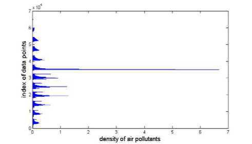
Figure1.              The distribution of air pollutants’ density

In Fig.1, the axis of abscissa shows the density of the air pollutants, and the ordinate shows the index of data points. From Fig.1 we can find that the range of air pollution density is from 0 to 7, the data value is mainly between 0 and 1, and the maximum is between 6 and 7.

To simulate the air pollutants we need to know their color and transparency. Because the color of air pollutants generally is gray, so the color information can be instead by the gray level information. The range of gray level is between 0 and 1. So we need to convert the data of density to the range of gray level. The mapping of conversion is:

f (x ) = z min (1) max - min

Where z is the concentration of data points, max and min are the maximum and minimum of density. Using (1) we can get the gray level of air pollutants about every measuring point. After the transformation the distribution of gray level becomes:

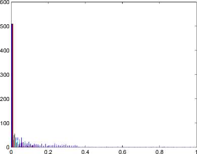
Figure2. The distribution of gray level.

From Fig.2 we can get the gray levels are mainly between 0 and 0.1, if we render the air pollutants according to the gray level in this range, the air pollutants will have large transparency. When we blend those gray levels with the city’s satellite image, the effect is not good enough and we can’t see any difference in most pixels between the emerged image and original image. This phenomenon is due to flaws of the processing of raw data. The regions with large pollution density are close to the monitoring points, and the data far away from the monitoring points are getting from the data interpolation so the value is smaller. We need to enhance the gray levels of air pollutants through the method of spatial domain image enhancement [2]. The equation of spatial domain image enhancement is:

x s = cr (2)

Where c is enhancement coefficient, r is the original gray level, x is power series, and s is the gray level after enhancement. If c=1the curves of (2) are as follows:

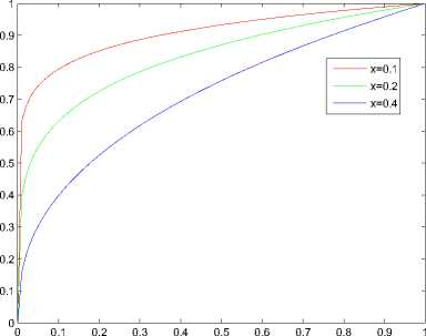
Figure3.            The curves of spatial domain image enhancement.

Processing the gray level according to (2), if x=0.2 we can get the following result:

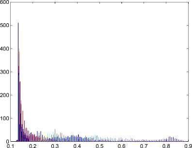
The distribution of gray level after enhancement.

Figure4.

Fig.4 shows the minimum of gray level increased, and the data value are distributed in each interval. The distribution of gray level becomes reasonable.

IV.    Color Surface Interpolation

There are only 9 air monitoring stations [11] in the whole city of Jinan, and each of them is far away from each other. So the air pollution data (data model) gathered from monitoring points is dispersive. We use B-spline surface interpolation [3][4][5] method to construct interpolation surface of gray level according to the discrete data points we had known. From the interpolation surface we can get the pollution density about any position of any resolution background image.

• A.    Compute the Control Points

If we want to construct interpolation surface, we should compute the control points first. The equation of computing the control points is:

m + j - 1 n + k - 1

p(ui + h , jk ) = E E dNК h ) N k (v j + k ) = p ,  (3)

i = 0 j = 0

Where p j ( i = 0,1, ™ , m ; j = 0,1, ™ , n ) are the colors of air pollutants, U = [ u 0 , u 1 , ™ , u_m + 2 h ] and V = [ v 0 , v 1 , ™ , v n _{+ 2} k ] are node vectors defined by:

u i = -pj—P ⁰ ,^ ( i = 0,1, ™ , m ; j = 0,1, ™ , n )

P m , j ^- P 0, j

V j = P ^— P i ,⁰ ( i = 0,1, ™ , m . j = 0,1, ™ , n )

P i , n ^- P i ,0

According (3) we can get the control points d_y(i = 0,1, ™ , m + h - 1; j = 0,1, ™ , n + k - 1).

But the solution process of (3) is complex. In this paper we convert the processing of computing control points into the following two-step [5]:

• 1)    According to the parameters U we construct n+1 B-spline curves as the section curves, the control points are d_ij ( i = 0,1, ™ , m + h - 1; j = 0,1, ™ , n ) , the equation is:

m+h-1___ q,(u+h) = EdN,h(ui+h)=Pj,(i=w,™’mj=0’1,"-’n)   (4)

i = 0

Through (4) we can get the control points d_ij .

2)    Along the direction of parameter v we interpolate the control points dij to construct the control curve ri (v):

Г ( V + k ) = E 1 d j N j,k (u j + k ) = d j ,( /’ = 0,1, " , n ; i = 0,1, ™ ; m ) (5) j = 0

Through (5) we can get the control points d ^( i = 0,1, ™ , m + h - 1; j = 0,1, ™ , n + k - 1), those are the ( m + h ) x ( n + k ) control points that we need to construct the B-spline interpolation surface.

• B.    Construct Interpolation Surface

According to the control points d_j(i = 03, ™ m + h - 1; j =QX ™ n + k - 1)   and node vectors

U = [ u 0 , u 1 , ™ , u_m + h + 1 ] and V = [ v 0 , V 1 , ™ , v n + k + 1 ] we define the h x kth tensor product B-spline surface: mn

Pu ^{v )} = EE d i N i , h ^{( u ) N} jk⁽ v\ u h ^ u ^ u m + 1 , v k ^ v ^ v n + 1   ⁽⁶⁾

i = 0 j = 0

In (3) (4) (5) (6), N _{i , h} ( u ) and N _{j , k} ( v ) are B-spline basis function defined by:

• 1    if u. <  u <  u

I                        I + 1

• 0 otherwise

  N i ,0 ( u ) =

  
  

  N i, p (u ) =

  
  

  u - U i

  
  

  u i + p ^- u i

  
  

  N, p - i ( u ) +

  
  

  u i + p + i ^- u ui + p + i ^- u i + i

  
  

  N i + i, p - i ( u )

  
  

  C. Surface Interpolation Results

  
  

  According to the above method we interpolate the data. If the gray levels are coming from the pollutants density directly without spatial domain image enhancement, the surface is like this ：

  
  
  

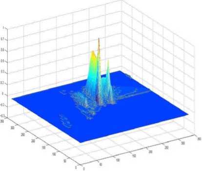
  Figure5. Interpolation surface of original data (1)

  
  
  

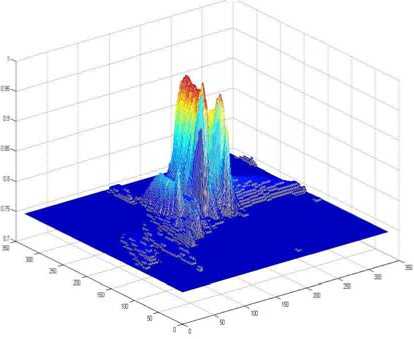
  Figure7.

  Interpolation surface of the data enhanced by

  
  
  

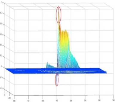
  Figure6. Interpolation surface of the original data (2).

  
  

  spatial domain(1).

  

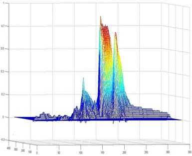
  Figure8.

  Interpolation surface of the data enhanced by

  spatial domain(2).

  
  

  There are some regions in the interpolation surface have quite difference after the spatial domain image enhancement. The surface cross-section of the region in which pollution data changes rapidly is like this:

  
  

  From Fig.5 and 6, we can see some value of points in the red circles is negative and some are significantly larger than others. The reason for this phenomenon is that the gray level converted from density changes intensely in some areas (a large value point closed to a small value point), so when we construct the interpolation surface according those points, the sharp points (negative points and large value points) are appeared. But the negative and large value points are not useful, so we use the method of spatial domain image enhancement to deal with the gray level.

  The method of spatial domain image enhancement has been mentioned in last section. After the data are enhanced, the interpolation surface become smoother, and the sharp points become fewer. Points become fewer. The surface is:

  
  
  
  
  

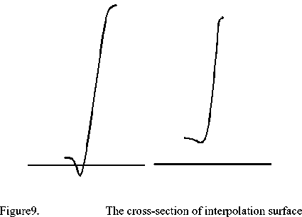
  The first curve is cross-section of the interpolation surface of original data. The curve goes through the negative region which is not what we need, and the large point of the curve is much larger than other points. The second curve is the same parts of the surface, but the surface is constructed according to the data that had been enhanced.

  
  

Figure11. The image rendering effects

V.    Rendering

• A.    Theoretical Basis

Air pollutants are emitted in to the air and form a layer of smog. If we consider an outdoor scene in daylight, smog will have mainly two effects: a drain of any color received by the eyes and a creation of veil of gray smog [5]. In this case, each pixel with color Cin drawn in the image is blended with the color of the fog C to obtain the final color : pollution                                                 fin f = f * Cin + (1 - f )* Cpolluion       (7)

Where coefficient f is the transparency of air pollutants those are obtained from the density of the air pollutants. In this paper we assumed them equal to the gray levels.

• B.    Original Background Image

We use satellite image of Jinan City as the background image of the experiment. Satellite images can truly reflect the topography of Jinan, and the experimental results are better than using other images. The satellite image is as shown in fig.10.

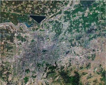
Figure10. Satellite image of Jinan

• C.    Rendering Result

  

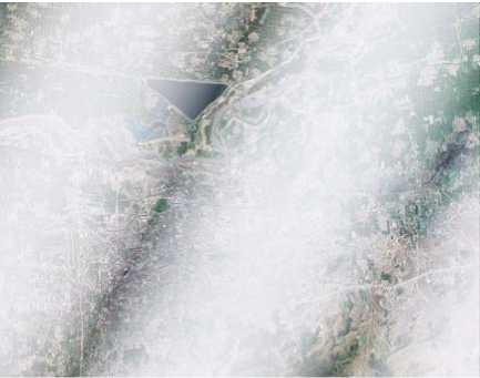
The air pollutants rendering result through image processing is as shown in Fig.11. In fig.11 we use randomly generated set of data to render the scene and do not use the existing air pollution data. Seen from the rendering result, the method can show that pollutants of different concentrations have different rendering results.

The visualization method mentioned in this paper can render the scenes through different viewpoints in the background of different resolutions. That is necessary for the system application in the network.

If we render the scenes according to the air pollution data in different resolution background images, the rendering results are:

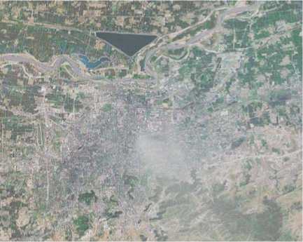
Figure12. Rendering result (resolutions are 1400×1200)

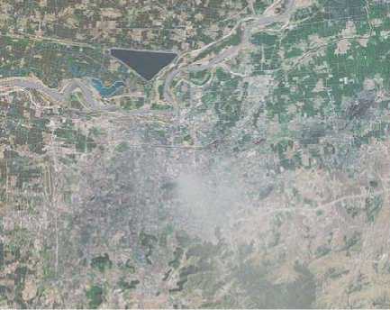
Figure13. Rendering results (resolutions are 700 X 600)

Fig.12 and Fig.13 show the rendering results in the different resolutions background image, and the resolutions are 1400 X 1200 and 700 X 600. This method is very important and favorable for the Internet transmission.

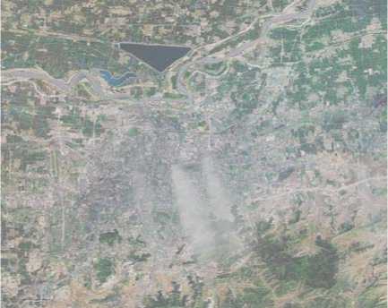
Figure14. The rendering result of air pollution data (1)

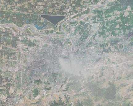
Figure17.            The rendering result of air pollution data (4)

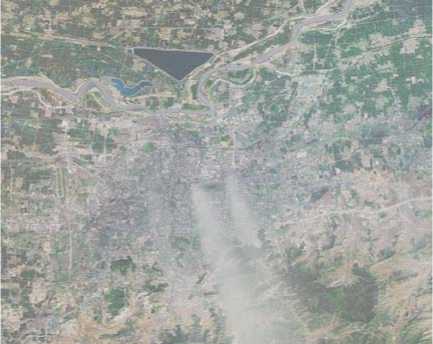
Figure15. The rendering result of air pollution data (2)

Fig.14, 15, 16 and 17 shows the rendering results of different data in the same background image. And the air pollution data is getting from the monitoring stations’ monitoring data at different time. From these four images we can see the changes of air pollutants shape and density at 4 different times. The darker regional has the larger density, and in the lighter area the density is smaller.

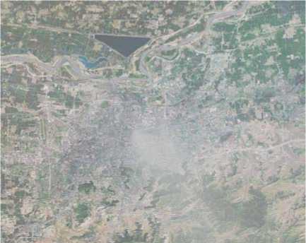
Figure16. The rendering result of air pollution data (3)

The method of scenes rendering presented in this paper supports the observation from different viewpoints. Suppose the previous view point is on the top of the scene. If we observe the scene from other view points, there should be different rendering effects. Because the data model is 3D data and the data is different seeing the model from different angles. To achieve that operation we process the data model from different directions and construct the interpolation surface following that direction, and then we can render the air pollutants according to the data obtain from the surface. Following this simple procedure we can render scenes for different viewpoints.

VI.    Conclusions

In this paper, we proposed a new method of air pollution data visualization based on image processing. The air pollution data is getting from the 9 monitoring stations in Jinan city. In the course of data processing, we use surface interpolation method to obtain a continuous density data according to the density of discrete data points. Interpolation surface would have some negative regions when the densities of adjacent two points change rapidly. In order to change this situation we have done a spatial domain image enhancement operation for those regions to make it changes smoothly. Through the surface interpolation we can achieve the rendering in background images of different resolutions.

In different light environments, air pollutants with the same density may show different effects and the transmission rate of the air pollutants itself is also slightly different. The above effects are to be implemented in the future.

Acknowledgment

First and foremost, I would like to show my deepest gratitude to my supervisor, Dr. Zhang, a respectable, responsible and resourceful scholar, who has provided me with valuable guidance in every stage of the writing of this thesis. Without his enlightening instruction, impressive kindness and patience, I could not have completed my thesis. I shall extend my thanks to Dr. Huang for all her kindness and help. I would also like to thank Dr. Weitao Li who has helped me to develop the fundamental and essential academic competence, and give me many Constructive comments in the thesis writing process.