Real Time Implementation of Audio Source Localization on Blackfin ADSP-BF527 EZ-KIT

Published Online July 2012 in MECS

Source localization is a fundamental problem in antenna array processing. It is based on exploiting the difference in propagation time between the received signals on a network of sensors to estimate their directions of arrival [1]. This area of research is of great interest in several branches, including radar systems, mobile radio communications, remote monitoring, sonar, geophysics and acoustic tracking. Thus, the everincreasing number of emerging applications involving the estimation of angles of arrival increases the requirements to develop more efficient methods as well as a number of sources to deal with localization accuracy and computation time. Many approaches have been developed to deal with the estimation of narrowband direction-of-arrival (DOA) estimation [1]–[8]. However, we find limited published works dealing with wideband sources. Some Pioneering works can be found in [9-12]. Two approaches are proposed to adopt narrow band processing techniques to that of wideband source cases. They are the incoherent aggregation technique [9], [10]-[11] and coherent signal subspace technique [12]. Furthermore, authors in [13] and [14] have reported a technique to span the signal and noise subspaces using spatio-temporal observation space. A generalization of the approach can be found in [15] that conduct to the spatial domain filter. Authors in [16]

have shown how to decompose the signal subspace into a modal decomposition in order to estimate the DOAs. Another interesting approach is reported in [17], it consists in using the maximum likelihood direction finding of wideband sources. Many real time implementations can be found in the literature. Most of them use an array of sensors. In this paper, only two sensors are used exploiting the stereo channel of the line-In board input. To enhance the performance obtained using such a reduced number of sensors, additional processing is required based mainly on audio activity detection before further processing of frames.

This paper is organized as follows; in section 2, the signal modeling is presented for narrow and wide-band sources, followed by multiple signal classification algorithm (MUSIC) description adapted to a wideband source. System components and implementation issues are discussed in section 3. In section 4, implementation results using recorded signals and real time signals are presented. At last, some concluding remarks are reported in section 5.

• II.    Signal ModelingA.    Narrow band versus wide band source signals

Consider the case of D narrowband sources emitting signals arriving at an array of sensors by the angles [0_T, ..., 0_k, ..., 0_D}. The signal received by the i^th sensor, Xi (t), is expressed by:

D

(t) = ^sk(t) e ~ i" ^ ^ ^ + n (t)        (1)

Where s_k(t) represents the signal from the k th source, ni (t) is the additive noise at the i^th sensor and T_j is the time lag between the received signal at the reference sensor С_г and Q. This delay is given by:

d{

T = — s in 0 v

Where d( is the distance between the sensors С_г and C j .

We also define the directional manifold vector for a set of M sensors as:

[                          ( М-1 ) sm0]

1е а …                ]

Thus, (1) can be rewritten as follows:

xt

( t )=∑ a_t ( 9k ) ^sk ( t )+ n_t ( t )

k=l

A wideband source consists of any signal whose energy is distributed across a wide frequency band. Localization methods like MUSIC algorithm have been developed for the case of narrow-band sources. Therefore, their application to wideband sources gave false results, mainly because these techniques exploit the fact that a signal delay in the time domain is transformed directly into a phase shift in the frequency domain, this allows us to write the received delayed source signal as:

s ( t -т)↔5( f ) _е-;2л:/т            (5)

We recall that a narrow-band source is characterized by a frequency bandwidth Δf very low relative to its central frequency fc , that is ∆ f ≪ fc .

The above condition conducts to deduce that the obtained phase shift is approximately constant throughout the occupied bandwidth, and the delayed signal can be expressed as:

s ( f ) _e-j2nfT =( f ) _e-j2Kf_c ^.1+^ /

≈( f ) _e-i2uf_CT ↔ s ( t ) _e-i2uf_CT (6)

Thus, the narrow-band sources are a special case where:

S ( f )= S ( f ) 8 ( f - fc )               (7)

If the bandwidth Δf is of the same order of value compared to the center frequency fc , s(t) is considered as a wideband. Hence, (6) and (7) are not true anymore. A common way to deal with the wide band signals is to consider the wide band signal as a combination of many narrow band signals fulfilling the approximations used in (6) and (7). The key feature of this method is to choose the frequencies owning the highest power. Indeed, if we analyze the spectrum of a wideband signal such as a speech signal, we can see that the latter has a significant power over a wide frequency range, and the existence of certain frequencies called "formants" where the concentration of energy is more important (see Figure (1)).

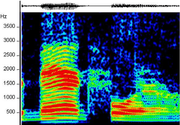
Fig 1: Spectrum of speech segment

Thus, the natural way to extend the methods dealing with the narrowband case to the wideband one is to treat separately each dominant frequency in the useful band and combine all the responses to obtain a comprehensive result.

• B.    Localization algorithm: Incoherent wide band

MUSIC (IWMUSIC)

The model in (4) can be rewritten in the frequency domain as follows:

X ( f , 9 )= A ( f , 9 ) S ( f )+ N ( f )       (8)

W e•re:   ( , )=[  ( , ),…,   ( , )]     is M dimensional vector containing the signals received at the M sensors.

• •    S ( f , 9 )=[ Si ( f , 9 ),…, S_D ( f , 9 )] т  is a D

dimensional vector of the emitting sources, assumed narrowband

• •    N ( f , 9 )=[ N₁ ( f , 9 ),…, Nm ( f , 9 )] т   is the

vector of additive noise disturbance of dimension M .

• •      ( ,  )=[ ( ,   ),…,  ( ,   )] is the

directional vector.

The autocorrelation matrix of the observation vector ( ,  ) is given by:

м

=  [     ]=1∑  ( , ) ( , )     (9)

М Z—i n=l

Where [.] is the expectation operator and {.} stands for conjugate transpose operator.

Replacing (8) in (9), we get:

( , )= ( , ) ( , ) ( , )+ (10)

Where ( , ) represents the source signal autocorrelation with dimension ( × ) and σI the noise correlation matrix of dimension ( × ).

The matrix is of a full rank (the eigenvectors are linearly independent); the Eigen decomposition can be written as:

=

• •    Matrix correlation computation (  , ) for each

of the dominant frequencies already selected for =1,2,…,  , where K is the number of dominant frequencies

• •    Subspace decomposition of each correlation matrix to separate the signal subspace from noise subspace and then calculate the spectrum of narrow-band MUSIC for each dominant frequency as follows:

^s™_s«(V.e) = _аЧГ,е)_ЕкЕ» _a(_f,_e)      ⁽¹²⁾

Where E_N of dimension M X (M — D) contains the eigenvectors of noise subspace.

• •    Averaging the K MUSIC spectra previously obtained:

к

P_№co_h⁽f, 6) = g а Н (_/к, dEEEEa^f_k, 0)  ⁽¹³⁾

• •    Estimation of direction of arrival of sources from the maxima of the resulting spectrum, already calculated using (13).

  =(    )( 0   ⁰ )(  )

  
  

  ̂=     [é(,)]        (14)

  
  

  =      +

  
  
  
  

Here, the matrix is a two partitioned matrix: the matrix    of dimension (×) with columns representing the Eigen vectors of the signal subspace and of dimension ×(-) contains the Eigen vectors of the noise subspace.

Finally, the IWMUSIC method involves the following steps:

• •    Overcoming the non-stationarity nature of the source, and this is done by segmenting the received signal into blocks of fixed size where a quasistationarity hypothesis holds.

• •    Conversion of the received temporal signal to the frequency domain

• •    Selection of the dominant frequencies (also known as formants or resonance frequencies) present in the spectrum by adaptive processing

• III. System Description

The studied algorithm was implemented on a fixed-point DSP using the SDK ADSP-BF527 EZ-KIT Lite [18] (CPU frequency 600 Mhz, 64 MB RAM, an audio codec with two inputs and two outputs, and an LCD display) using the VisualDSP++ software environment [19]. In this section, we describe all the operations carried out to implement the full system.

• A.    Microphones

We used two microphones connected to the Line-In input of the development board. The acquired signal is sent through the mono/stereo converter as depicted in Figure 2; it allows us to exploit a stereo channel as two independent mono channels. Hence, our system uses only two sensors for locating one audio source.

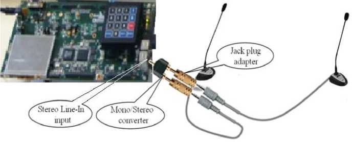
Fig 2: Data Acquisition via two microphones

The two microphones are omni-directional, and powered by batteries 1.5Volts; they have a flat frequency response in the frequency range 50-18000Hz, which is favorable to audio applications. To transfer the data in real time, we used the codec BF527C1 integrated into the development board ADSP-BF527 EZ-KIT Lite that is described in the following paragraph.

• B.    Audio codec BF527C1

This codec has good performance and features quite satisfactory for applications using audio. Indeed, it has an analog/digital and digital/analog converter with sampling rates from 8 kHz to 96 kHz and encoding precision of 16 to 32 bits.

The transfer of data between the codec and the processor is done through the serial port SPORT0 via

DMA controller, and the internal registers of the codec are set by the processor through the SPI or TWI's depending on the choice of the user, while the data is transferred to memory via two protocols: LJ or I2S.

In our case, we configured the audio codec using the TWI interface to run with the serial port SPORT0 where is connected. The data transfer is done from the serial port to a reserved area of memory through the DMA controller. Buffers for each channel of the codec are continuously filled and emptied by the DMA controller. So, the CPU must have a relatively high processing speed, compared to the data transfer, to avoid conflicts due to concurrency over the same data by the CPU and DMA controller [20].

To circumvent this problem, we used a simple technique called "Ping-pong," which isolates the CPU activity to that of DMA.

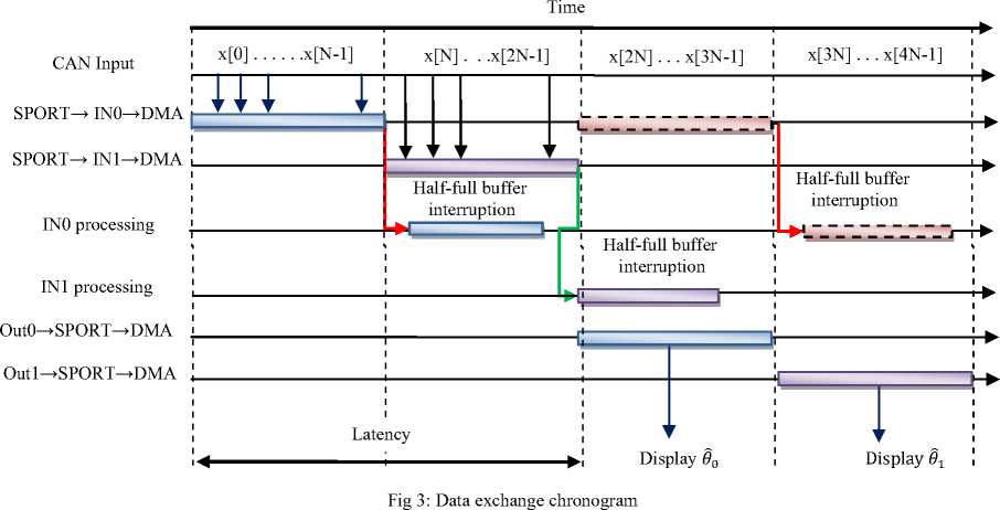
• C.    Frames processing using "Ping-Pong" technique

This technique is illustrated in Figure 3. Firstly, a buffer of length 2 x N is created (where N is the block size of data to process). The latter is itself divided into two buffers of length N: IN0 (Ping) and IN1 (Pong). The processing of the buffer IN1 is performed in parallel with the filling of the buffer IN0 by the DMA controller, once the filling of IN0 and IN1 operation ends, the situation is reversed: the DMA controller starts filling the buffer IN1 while the processor processes the data in the buffer IN0 and so forth.

In general, the acquisition process illustrated through the timing diagram of figure 3 can be summarized as follows: the program starts by setting up the DMA registers and the serial port. When completed, the DMA controller begins acquiring data from the SPORT and put them in a buffer memory which is divided into two buffers IN0 and IN1. The data is sent to the IN0 buffer at the beginning, once it is full, the DMA controller generates an interrupt to start processing the data buffer IN0 and switch IN1 filling the buffer, and thus the Pingpong technique linked together as explained in the preceding paragraph.

For storage and serial transmission of the processed results, two other buffers of length N: OUT0 and OUT1 must be created in the same way. The transmission of processed data toggles between the two buffers as shown in figure 3. Usually the result of processing IN0 is sent to the buffer OUT0 and serial transmission of the latter is performed in parallel with the treatment of IN1 and vice versa. The IN0 processing is done simultaneously with serial transmission of data stored in OUT1 .

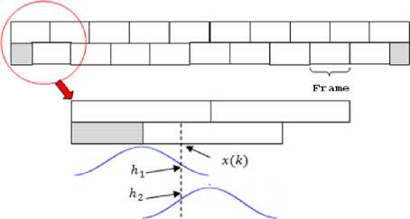
• D.    Windowing operation

Each frame of the signal is weighted by a Hamming window with 50% overlap. The sample у(к) will be weighted according to (15):

у (к) = h1x(k) + ft2 (W

Figure 4 depicts the practical procedure of windowing.

• E.    Processing implementation issues

During real-time tests in reverberant environment (laboratory), the used source is a speaker sending an audio signal to two microphones placed at a variable distance. After some testing, and through the results displayed on the LCD, we found that the displayed estimated angles were very volatile and often erroneous due to various disturbances such as multiple reflections suffered by signals through the soil and walls.

In addition, a speech signal is mainly composed of voiced sound and unvoiced one. The spectrum of the first is characterized by the presence of formants where the incoherent method is justified, while the spectrum of the latter is smooth (no maximum energy) and therefore, the application of the method is no longer justified.

• a. Proposed solution: Voice Activity Detection

To solve the above problem, we propose to use an audio activity detector immediately after sample acquisition. It consists on computing the energy and a zero crossings rate (ZCR) to distinguish frames of voiced sound from the unvoiced ones [21].

The voiced sound, which generally corresponds to the pronunciation of vowels, is characterized by a relatively constant frequency, and therefore, has a lower ZCR.

The unvoiced speech is non-periodic and a noise-like signal; it is characterized by a high ZCR. The ZCR is computed as follows:

- У ISgn[x(m)] - Sgn[x(m -

N Z—i

m=0

1)]1    (16)

Where   Sgn[x(n)] = { —S1x(^) > 0     and n

-1 5 i x(n) < 0

represent the frame length.

The energy of a signal is another parameter used to distinguish between the voiced/unvoiced speech. The energy is calculated as follows:

N-l

Eu =y|x(m)|2              (17)

m=0

The appropriate method to distinguish between the voiced and unvoiced is illustrated in the diagram depicted in Figure 5 where the unvoiced part is considered as noise. Hence, it is discarded from processing.

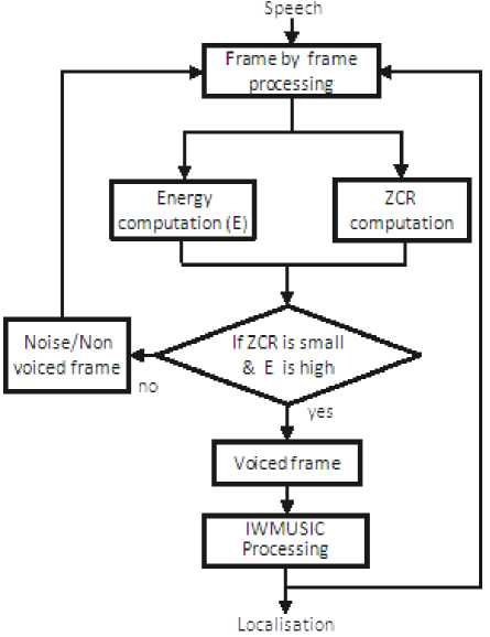
Fig 5: Block diagram of the voiced/unvoiced classification

Figure 6 shows the ZCR histograms calculated for frames of 256 samples for a background noise (in blue) and the speech signal (red). As we can see from figure 7, we can set up a threshold to differentiate between voiced sounds (red) and unvoiced sounds (blue).

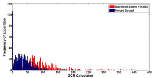
Fig 6: Distribution of zero-crossings for unvoiced and voiced speech

• F.    Spectrum computation

After selecting useful frames, we compute their spectrum. This operation is done thanks to the function rfft_fr16 available in the VisualDSP++ library filter.h . It is an optimal function developed in assembly language. The function accepts data in Q1.15 format, and calls another function twidfftrad2_fr16 to obtain twiddle factors [19].

• a. Adaptive selection of dominant frequencies

After the FFT computation, we take the magnitude of the spectrum. To select dominant frequencies, an adaptive threshold is used depending on the required number of frequencies to be analyzed. To this end, the spectrum is divided into several intervals depending on how many dominant frequencies to be extracted, then one carries out the search for the maximum of each interval. The threshold is set based on the number of frequencies to be extracted, and the values below this threshold will be set to zero.

The following steps summarize the operations for frequency selection.

• •    Fourier transform computation S(f)

• •    Power spectral computation |S(f)| ²

• •    Subdivide the spectrum into intervals and search the local maxim within every interval

• •    Save indices of maxima in a vector

• •    Set a threshold less then the obtained maxima

• •    Set to zero all the values of spectrum less then the threshold

Magnitude

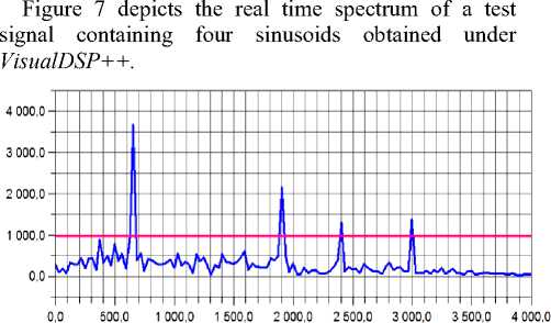
Frequency (Hz)

Fig 7 : Signal spectrum with adapted threshold

• G.    Singular values decomposition

The time samples are projected into the frequency domain by Fourier transform, then computes the modulus of the obtained complex spectrum to extract the four dominant frequencies corresponding to the maxima of the latter.

We define dominant frequency for each observation a complex matrix of dimension (N × M) (where N is the number of points taken around each dominant frequency and M is the number of used sensors). Then, instead of decomposing the correlation matrix into its own elements (EVD), it is interesting to decompose the complex matrix of observations in singular values elements (SVD), and this, to separate the signal subspace from the noise subspace [22].

This is the heart of the MUSIC algorithm because it allows the separation of the noise subspace from the signal subspace.

Note that this algorithm is applied to real matrices. To apply it to the complex matrix of observations, we used a technique to convert a complex matrix ( A + iB ) in a real matrix ( A, B, -B, A ) such that: real matrices A and B are obtained from the real and imaginary parts of the complex matrix [23], using the following transformation equations:

(Л + IB )(u + iv) = w(u + iv) (18)

[Д M-K1 (19)

This means that if W i , w₂, —, W_N are the Eigen-values of the complex matrix ( A + iB ). Then the Eigen-values of the real matrix of (19) will be Wi, Wi,w₂, W₂ ..., w_N,w_N, , and all pairs of eigenvectors (u + iv) and i (u + iv) correspond to the same Eigen-value [24].

In our case, the complex matrix of observations is of dimension (2 × 2) because we have two sensors and two frequency samples around each dominant frequency were taken.

The results of the implementation of this algorithm are detailed in the Table 1 for a real matrix of size (4×4), with an accuracy of 10-5, the number of total cycles required to calculate the incoherent MUSIC spectrum is roughly equal to four times the computing time of a single matrix, and this, of course, in case we select four dominant frequencies from the spectrum.

Table 1: DSP implementation results

Function	CPU cycles number	Time execution ( ? ? s)	Occupied Memory (words of 32bits)
FFT	68723	114.53	157
Adaptive selection of each dominant frequency	95531	159.21	288
Adaptive selection of four dominants frequencies	164254	273.74	455
One SVD decomposition matrix	132140	220.24	4752
Total (four decompositions)	528560	880.96	4752
One steering vector computation	178118	296.86	238
Four steering vectors computation	712472	1187.44	238
Narrowband Music spectrums computation	638455	1064.09	366
Incoherent averaging of Pseudo spectrums	44544	74.24	134
DOA estimation	727345	1138.33	500

To compute the pseudo-spectrum of narrow-band MUSIC, we need to compute the directional vector. The following steps are conducted:

• •    For each fl , we compute л

( Я depends also on t ℎ e distance d)

• •    Set « For » loop for angles 6 =-90 ; Set i =0

• •    Compute a ( i ) = ^j27idsin0 ^/2 and a^H ( i ) =

g-j27idsin0 /Я

• • e++ ;i++

• •    If 6 =90 , go next step otherwise go step 2

• •    Compute the spectrum of narrow-band MUSIC for each dominant frequency

H. Dispalying results on LCD VaritronixMCQB01 screen

To view the results of the estimated angle of arrival, we used the LCD display contained in the developing board. For this, the LCD display is configured to operate in parallel with the audio codec.

This display is controlled by a Xilinx CPLD and connected to the parallel interface "PPI". VisualDSP + + software has several predefined functions that allow full configuration of the display. The steps for configuring the LCD are as follows [25]:

• •    Open the display by using the adi_ssl_init () function.

• •    Open the parallel interface "PPI".

• •    Configure the PPI’s control register to work with the LCD

• •    Configure the mode of data buffering.

• •    Define the addresses of the LCD image buffers.

• •    Activate the flow of image data to the display.

Each time the algorithm is executed; the result is displayed on the screen with a number and a needle scanning a portion of a semicircle to locate the sound source in space. To do this, we created a library containing the decimal digits from '0 'to '9' and the '+' and '-' signs, each character is considered as a matrix of (19 × 19) pixels containing only '1 'or '0' bits.

A snapshot of one of the AOA estimation is shown in Figure 8.

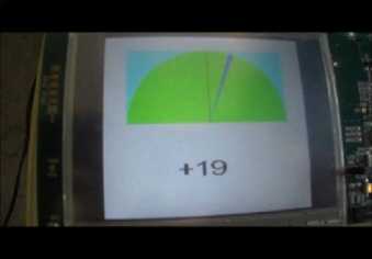
Fig 8: Displaying source localization result on LCD screen

• IV.    Experimental ResultsA.    Parameters’ influence

Before moving on real time implementation tests, we made several Monte Carlo simulations consisting on plotting the deviation of the estimated direction of arrival from the true direction of arrival for different values.

We used two signals: a speech signal and a wideband signal obtained by summing four sine waves of frequencies: 600 Hz, 1400 Hz, 2200 Hz and 3000 Hz. The results are depicted in figure 9.a for a combination of 4 pure frequencies and in figure 9.b for a recorded speech signal.

In general, we see better results while increasing the SNR. We also note that using a signal consisting of four sinusoids gives deviations lower than those obtained using a speech signal. Because the first signal exactly verifies the hypothesis of incoherent summation method that assume all relevant information of a signal is concentrated in only a few frequencies, while for a speech signal, the energy (and therefore, useful information) is distributed over the entire band, and it is not completely concentrated on some formants.

In addition, to see the influence of the number of selected frequency components, we repeated the previous simulations with the same speech signal, but by selecting only three frequencies (see figure 10.a), and only selecting two frequencies (see figure 10.b).

We find that the decrease in the number of selected frequencies requires higher SNR to achieve a good estimation of angles of arrival.

• B.    Implementation resources

The results of the implementation of this algorithm, in terms of the execution time and used memory space, are summarized in the Table 1.

We point out that the number of cycles performed in each arithmetic operation cannot be known exactly as an iterative method is used whose convergence time varies from one array to another.

For real-life signals, the developed system is tested in reverberant room. The obtained results fluctuate dramatically in the LCD display. In fact, the displayed values seem to take random values. Hence, the VAD, described in section III (subsection E), is inserted in the system, and values’ averaging over few frames is carried out before displaying an estimated result. We repeated the experiments. These new modifications have yielded more stable results. Figure 11 depicts the obtained angle deviation performance; each plotted value represents an average of 100 measurements taken.

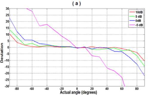
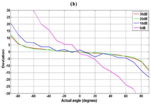
Fig 9: Angle deviation versus SNR.

• V.    Conclusion

In this paper, a real time implementation of audio source localization is described. The used algorithm is based on the generalization of MUSIC technique to deal with wideband sources. The conducted steps are described, and details of implementation issues are provided. Furthermore, to deal with the volatility of the displayed estimated angles of arrivals, we suggested inserting audio activity detection before going on further processing. Moreover, values’ averaging over few frames is done to stabilize the results. Real time tests have been conducted for the localization of a single acoustic source in a reverberant environment using only two sensors. The results obtained in real time are promising for such a reduced number of sensors. Indeed, multiple reflections, the lack of perfect symmetry of the sensors, and the assumption of plane wave are influenced the results provided by the algorithm in real time. To enhance the localization, more sensors should be used.

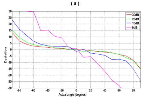
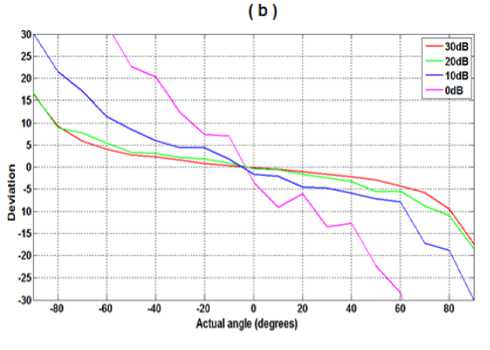
Fig 10: Number of selected frequencies versus SNR

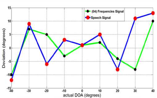
Fig 11: Deviation of Estimated DOA from Actual DOA.