Reducing Support Vector Machine Classification Error by Implementing Kalman Filter

Author: Muhsin Hassan, Dino Isa, Rajprasad Rajkumar, Nik Ahmad Akram, Roselina Arelhi
Journal: International Journal of Intelligent Systems and Applications(IJISA) @ijisa
Article in issue: 9 vol.5, 2013.
Free access
The aim of this is to demonstrate the capability of Kalman Filter to reduce Support Vector Machine classification errors in classifying pipeline corrosion depth. In pipeline defect classification, it is important to increase the accuracy of the SVM classification so that one can avoid misclassification which can lead to greater problems in monitoring pipeline defect and prediction of pipeline leakage. In this paper, it is found that noisy data can greatly affect the performance of SVM. Hence, Kalman Filter + SVM hybrid technique has been proposed as a solution to reduce SVM classification errors. The datasets has been added with Additive White Gaussian Noise in several stages to study the effect of noise on SVM classification accuracy. Three techniques have been studied in this experiment, namely SVM, hybrid of Discrete Wavelet Transform + SVM and hybrid of Kalman Filter + SVM. Experiment results have been compared to find the most promising techniques among them. MATLAB simulations show Kalman Filter and Support Vector Machine combination in a single system produced higher accuracy compared to the other two techniques.
Discrete Wavelet Transform (DWT), Support Vector Machine (SVM), Kalman Filter (KF), Defect classification
Short address: https://sciup.org/15010460
IDR: 15010460
Text of the scientific article Reducing Support Vector Machine Classification Error by Implementing Kalman Filter
Published Online August 2013 in MECS
Support Vector Machine is a popular method used for classification and regression in modern days [1]. SVM gains popularity as an alternative for Artificial Neural Networks due to its superior performance [1]. This improvement is due to structural risk minimization used in SVM. Structural Risk Minimization is proven better generalization ability compared to ANN’s empirical risk minimization technique [1].
Application of SVM in pipeline fault diagnosis shows a promising future [2]. For instance, one can teach SVM to classify type of defect in given situation. This will help with monitoring and classification of what type of defect happen in the time of experiment. In a previous experiment, different type of defects with varying depths simulated in the laboratory has been classified using SVM. Datasets used in this experiment have been added with Additive White Gaussian Noise to study the performance of hybrid technique for SVM, namely Kalman Filter + SVM hybrid combination [3]. In practical scenario, datasets obtained from the field are susceptible to noise from an uncontrollable environment. This noise can greatly degrade the accuracy of SVM classification. To maintain the high level of SVM classification accuracy, a hybrid combination of KF and SVM has been proposed to counter this problem. Kalman Filter will be used as a pre-processing technique to de-noise the datasets which are then classified using SVM. A popular de-noising technique used with Support Vector Machine to filter out noise, the Discrete Wavelet Transform (DWT) is included in this study as a benchmark for comparison to the KF+SVM technique. Discrete Wavelet Transform is widely used as SVM noise filtering technique [4][5]. DWT has become a tool of choice due to its time-space frequency analysis which is particularly useful for pattern recognition [6]. In this paper, KF+SVM combination shows promising results in improving SVM accuracy. Even though Kalman Filter is not widely used for de-noising in SVM compared to DWT, it has the potential to perform as a de-noising technique for SVM. In previous experiment, each technique tested has been fed with each separate added noise datasets respectively. However in this paper, the performances of these three techniques (SVM vs. DWT+SVM vs. KF+SVM) with the same noisy datasets input will be tested and compared in Results and Discussion section. A more detailed difference of previous paper and this paper workflow is available at Methodology section.
-
II. Background
2.1 Pipeline -
2.2 Support Vector Machine
Corrosion is a major problem in offshore oil and gas pipelines and can result in catastrophic pollution and wastage of raw material [7]. Frequent leaks of gas and oil due to ruptured pipes around the world are calling for the need for better and more efficient methods of monitoring pipelines [8]. Currently, pipeline inspection is done at predetermined intervals using techniques such as pigging [9]. Other non-destructive testing techniques are also done at predetermined intervals where operators must be physically present to perform measurements and make judgments on the integrity of the pipes. The condition of the pipe between these testing periods, which can be for several months, can go unmonitored. The use of a continuous monitoring system is needed.
Non Destructive testing (NDT) techniques using ultrasonic sensors are ideal for monitoring pipelines as it doesn’t interrupt media flow and can give precise information on the condition of the pipe wall. Long range ultrasonic testing (LRUT) utilizes guided waves to inspect long distances from a single location [10]. LRUT was specifically designed for inspection of corrosion under insulation (CUI) and has many advantages over other NDT techniques which have seen its widespread use in many other applications [11]. It is also able to detect both internal and external corrosion which makes it a more efficient and cost-saving alternative. With the recent developments in permanent mounting system using a special compound, the ability to perform a continuous monitoring system has now become a reality [12].
An LRUT system was develop in the laboratory for 6 inch diameter pipes using a ring of 8 piezo-electric transducers [13]. Signals were acquired from the pipe using a high speed data acquisitions system. The developed LRUT system was tested out using a section of a carbon steel pipe which is 140mm in diameter and 5mm thick. A 1.5m pipe section was cut out and various defects were simulated as shown in Table 1. A full circumferential defect with 3mm axial length was created using a lathe machine. Depths of 1mm, 2mm, 3mm and 4mm were created for this defect and at each stage tested using the LRUT system.
Guided wave signals have been used for many researchers by utilizing different signal processing techniques as a means of identifying different types and depths of defects. Advanced signal processing techniques such as neural networks have also been used to quantify and classify defects from the guided wave signals [14] [15]. Since neural networks are a supervised learning algorithm, the data required for its training phase from are obtained from simulation methods. Simulation is performed by modeling the damage based on reflection coefficients or finite elements [16]. The trained neural network model is then tested from data obtained experimentally and have shown to obtain very good accuracy in classifying defects in pipes, bars and plates [17].
Support vector machines, founded by V. Vapnik, is increasingly being used for classification problems due to its promising empirical performance and excellent generalization ability for small sample sizes with high dimensions. The SVM formulation uses the Structural Risk Minimization (SRM) principle, which has been shown to be superior, to traditional Empirical Risk Minimization (ERM) principle, used by conventional neural networks. SRM minimizes an upper bound on the expected risk, while ERM minimizes the error on the training data. It is this difference which equips SVM with a greater ability to generalize [18].
Given a set of independent and identically distributed (iid) training samples, S={(x1, y1), (x2, y2),…..(xn,yn)}, where xi∈ RN and yi∈ {-1, 1} denotes the input and the output of the classification, SVM functions by creating a hyperplane that separates the dataset into two classes. According to the SRM principle, there will just be one optimal hyperplane, which has the maximum distance (called maximum margin) to the closest data points of each class as shown in Fig. 1. These points, closest to the optimal hyperplane, are called Support Vectors (SV). The hyperplane is defined by (1), w∙X+b =0 (1) and therefore the maximal margin can be found by minimizing (2) [18].
-
| ‖w‖2 (2)
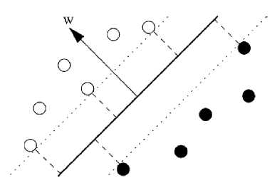
Fig. 1: Optimal Hyperplane and maximum margin for a two class data
The Optimal Separating Hyperplane can thus be found by minimizing (2) under the constraint (3) that the training data is correctly separated [20].
У/∙(Xi ∙w+b)≥1,∀i (3)
The concept of the Optimal Separating Hyperplane can be generalized for the non-separable case by introducing a cost for violating the separation constraints (3). This can be done by introducing positive slack variables ξ i in constraints (3), which then becomes,
У/∙(xt ∙w+b)≥1-^t ,∀i (4)
If an error occurs, the corresponding i must exceed unity, so S i ^ i is an upper bound for the number of classification errors. Hence a logical way to assign an extra cost for errors is to change the objective function (2) to be minimized into:
min{|^^2+ О(£^)) (5)
where C is a chosen parameter. A larger C corresponds to assigning a higher penalty to classification errors. Minimizing (5) under constraint (4) gives the Generalized Optimal Separating Hyperplane. This is a Quadratic Programming (QP) problem which can be solved here using the method of Lagrange multipliers [21].
After performing the required calculations [18, 20], the QP problem can be solved by finding the LaGrange multipliers, αi, that maximizes the objective function in (6), n1
W («) = S a - S aa j^y (xi xj)
i = 1 2 i , j = 1
subject to the constraints,
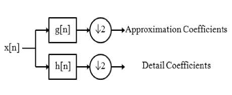
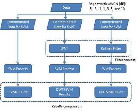
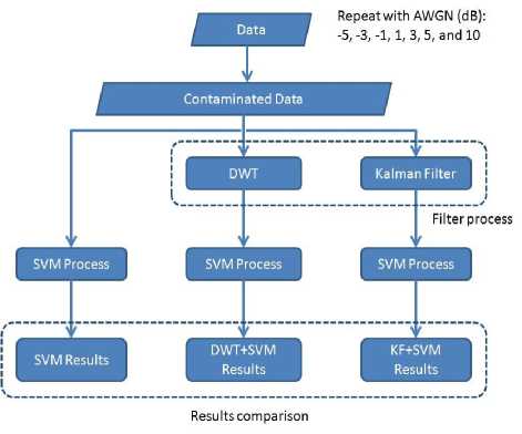
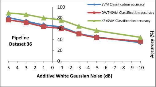
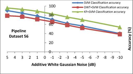
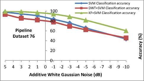
O^a The new objective function is in terms of the Lagrange multipliers, αi only. It is known as the dual problem: if we know w, we know all αi. if we know all αi, we know w. Many of the αi are zero and so w is a linear combination of a small number of data points. xi with non-zero αi are called the support vectors [22]. The decision boundary is determined only by the SV. Let tj (j=1, ..., s) be the indices of the s support vectors. We can write, s w=S а-,У<Л (8) j=1 So far we used a linear separating decision surface. In the case where decision function is not a linear function of the data, the data will be mapped from the input space (i.e. space in which the data lives) into a high dimensional space (feature space) through a non-linear transformation function Ф ( ). In this (high dimensional) feature space, the (Generalized) Optimal Separating Hyperplane is constructed. This is illustrated on Fig. 2 [23]. Fig. 2: Mapping onto higher dimensional feature space By introducing the kernel function, K (x., xj)=^( xi), ф( xj)), (9) It is not necessary to explicitly know Ф ( ). So that the optimization problem (6) can be translated directly to the more general kernel version [23], nn W(a) = Sai-^ S aiajyiyjK(X,xj) (10) i=1 2i=1, j=1 n subject to c > a > o,S aУг = о. i=1 After the αi variables are calculated, the equation of the hyperplane, d(x) is determined by, l i=1 The equation for the indicator function, used to classify test data (from sensors) is given below where the new data z is classified as class 1 if i>0, and as class 2 if i<0 [24]. iFC^) = si^n[d(x)] = si^n[Z=1yiaiK(x,xi) +b] (12) Note that the summation is not actually performed over all training data but rather over the support vectors, because only for them do the Lagrange multipliers differ from zero. As such, using the support vector machine we will have good generalization and this will enable an efficient and accurate classification of the sensor signals. It is this excellent generalization that we look for when analyzing sensor signals due to the small samples of actual defect data obtainable from field studies. In this work, we simulate the abnormal condition and therefore introduce an artificial condition not found in real life applications. Kalman Filter is named after Rudolf E. Kalman who invented this algorithm in 1960. In the past, Kalman Filters have been a vital implementation in military technology navigation systems for missiles (navigation system for nuclear ballistic missile submarines, guidance and navigation systems of cruise missiles such as U.S Navy’s Tomahawk missile and the U.S Air Force’s Air Launched Cruise Missile and guidance for NASA Space shuttle [25][26][27]. Even though Kalman Filter is not widely used for de-noising in SVM compared to DWT, it has the potential to perform as denoising technique for SVM as shown by Huang in online option price forecasting for stocks market experiment [28] and by Lucie Daubigney and Oliver Pietquin in single trial p300 detection assessment [29]. In both papers, Kalman filter show a promising results in de-noising the noise before it being fed into SVM. G. Welch and G. Bishop [30] define Kalman Filter as “set of mathematical equations that provides an efficient computational (recursive) means to estimate the state of a process, in a way that minimizes the mean of the squared error”. According to Grewal and Andrews [31], “Theoretically Kalman Filter is an estimator for what is called the linear-quadratic problem, which is the problem of estimating the instantaneous “state” of a linear dynamic system perturbed by white noise – by using measurements linearly related to the state but corrupted by white noise. The resulting estimator is statistically optimal with respect to any quadratic function of estimation error.” In layman term, “To control a dynamic system, it is not always possible or desirable to measure every variable that you want to control, and the Kalman Filter provides a means for inferring the missing information from indirect (and noisy) measurements. The Kalman filter is also used for predicting the likely future courses of dynamic system that people are not likely to control” [31]. Equation for a simple Kalman Filter given below [32]: For a linear system and process model from time k to time k+1 is describe as: xk+1 = Fxk+Guk+wk(13) where xk, xk+1 are the system state (vector) at time k, k+1. F is the system transition matrix, G is the gain of control uk, and wk is the zero-mean Gaussian process noise, w ~ N(0, Q) Huang suggested that for state estimation problem where the true system state is not available and needs to be estimated [30]. The initial xo is assumed to follow a known Gaussian distribution Xo ~ N(CCO, P ) . The objective is to estimate the state at each time step by the process model and the observations. The observation model at time k+1 is given by. zk+1 = Hxk+1 + vk+1 Where H is the observation matrix and vk+1 is the zero-mean Gaussian observation noise vk+1~N (0, R). Suppose the knowledge on xk at time k is xk ~ N(xk, Pk ) Then xk+1 at time k+1 follow x,+1~ N (x. +1, Pk+1) where ̂ , Pk+1 can be computed by the following Kalman filter formula. Predict using process model: xk+1 = Fxk+Guk Pk+1 = FPkFT + Q Update using observation: xk+1 = xk+1 + K(Zk+1 - Hxk+1)(19) Pk+1 = Pk+1 + KSKT(20) Where the innovation covariance S (here- ̅ is called innovation) and the Kalman gain, K are given by S = HPk+1HT + R(21) K = Pk+1HTS-1 A discrete wavelet transform (DWT) is basically a wavelet transform for which the wavelets are sampled in discrete time. The DWT of a signal x is calculated by passing it through a series of filters. First the samples are passed through a low pass filter with impulseresponse g, resulting in a convolution of the two (23). The signal is then decomposed simultaneously using a high-pass filter h (24). ю yiow [n ]= S x[k]g [2n - k] (23) k=—^ ^ Ул/gh[n ]= S x[k ]h [2 n — k ] (24) k=—^ The outputs of equations (23) and (24) give the detail coefficients (from the high-pass filter) and approximation coefficients (from the low-pass). It is important that the two filters are related to each other for efficient computation and they are known as a quadrature mirror filter [33]. However, since half the frequencies of the signal have now been removed, half the samples can be discarded according to Nyquist’s rule. The filter outputs are then down sampled by 2 as illustrated in Fig.3 [34]. This decomposition has halved the time resolution since only half of each filter output characterizes the signal. However, each output has half the frequency band of the input so the frequency resolution has been doubled [34]. The coefficients are used as inputs to the SVM [35]. Fig. 3: DWT filter decomposition [34] In this paper, a revision has been made to my previous experiment [3]. The same pipeline dataset was used, however in this experiment the additive white Gaussian noise added to the dataset is the same for all three techniques. This means that now, all the techniques have the same set of dataset contaminated with noise (refer to Fig.5). In previous experiment, the noisy dataset for each technique is added respectively to each technique as shown in Fig.4. Using the flowchart above, it is a more reliable comparison between SVM, DWT+SVM and KF+SVM to use the same contaminated data. For SVM technique, the data runs through SVM to see the performance of SVM and this will be use as benchmark. For DWT+SVM, the data is first filter using DWT techniques before the filtered-data used as input for SVM. The same goes for KF+SVM techniques whereby the data is first filter using Kalman Filter in this case and the filtered-data used as input for SVM. Fig. 4: Flowchart of previous works to obtained comparison of SVM, DWT+SVM and KF+SVM accuracy Fig. 5: Flowchart of current works to obtained comparison of SVM, DWT+SVM and KF+SVM accuracy The basic technique for SVM classification is good enough to classify pipeline defect, however the problem arises when several tests which include AWGN into the data to mimics noise in real application show that noise can greatly affect the SVM accuracy. In MATLAB tests, AWGN values used are from 5dB to -10dB. In this proposed solution, additive white Gaussian noise (AWGN) has been added using function in MATLAB. AWGN is widely use to mimics noise because of its simplicity and traceable mathematical models which are useful to understand system behavior [36][37]. Figures below show classification accuracy results of SVM, DWT+SVM and KF+SVM for pipeline dataset 36, 56 and 76. In all datasets results, KF+SVM show a better classification accuracy results compared to SVM or DWT+SVM. KF+SVM managed to be by average 10% more accurate than SVM and DWT+SVM techniques. In previous paper [3], the KF+SVM average results is above 90% in all additive white Gaussian noise level even for the case of -10dB of AWGN using the different contaminated data for each techniques. For this experiment using the same contaminated data, it is found that by average, KF+SVM is producing at least 10% higher than SVM or DWT+SVM classification accuracy results. Fig. 6: Comparison results between SVM, DWT+SVM and KF+SVM for dataset 36 Fig. 7: Comparison results between SVM, DWT+SVM and KF+SVM for dataset 56 Fig. 8: Comparison results between SVM, DWT+SVM and KF+SVM for dataset 76 This experiment using the same contaminated datasets for all three techniques show different results from previous experiment where the contaminated datasets for each technique was added separately. In this experiment, SVM accuracy results is slightly better than DWT+SVM, while KF+SVM technique is still proven a better choice to improve classification accuracy. However the improvement done by KF+SVM is roughly only 10% better than the other two techniques whereby in previous experiment KF+SVM managed to maintain a consistent above 90% classification accuracy in all AWGN noise level. We come to conclusion that this is a more suitable way to run the experiment, by using the same contaminated datasets for all techniques used. It gives a more accurate benchmark results comparison for this experiment. I would like to thank, Ministry Of Science, Technology and Information (MOSTI) Malaysia for sponsoring my PhD. I also like to extend my gratitude to Prof. Dino Isa and Dr. Rajprasad for providing the pipeline datasets for the MATLAB simulations and Nik Akram for his help in this project. [1] Ming Ge, R. Du, Cuicai Zhang, Yangsheng Xu, “Fault diagnosis using support vector machine with an application in sheet metal stamping operations”. Mechanical Systems and Signal Processing 18, 2004, pp. 143-159. [2] D. Isa, R. Rajkumar, KC Woo, “Pipeline Defect Detection Using Support Vector Machine”, 6th WSEAS International conference on circuits,systems, electronics, control and signal processing, Cairo, Egypy, Dec 2007. pp.162-168. [13] Dino Isa, Rajprasad Rajkumar, “Pipeline defect prediction using long range ultrasonic testing and intelligent processing” Malaysian International NDT Conference and Exhibition, MINDTCE 09, Kuala Lumpur, July 2009. [14] Rizzo, P., Bartoli, I., Marzani, A. and Lanza di Scalea, F.,“Defect Classification in Pipes by Neural Networks Using Multiple Guided Ultrasonic Wave Features Extracted After Wavelet Processing”, ASME Journal of Pressure Vessel Technology. Special Issue on NDE of Pipeline Structures, 127(3), 2005, pp. 294-303. [15] Cau F., Fanni A., Montisci A., Testoni P. and Usai M., “Artificial Neural Network for NonDestructive evaluation with Ultrasonic waves in not Accessible Pipes”, In: Industry Applications Conference, 2005. Fortieth IAS Annual Meeting, Vol. 1, 2005, 685-692. [16] Wang, C.H., Rose, L.R.F., “Wave reflection and transmission in beams containing delamination and inhomogeneity”. J. Sound Vib. 264, 2003, pp.851– 872. [17] K.L. Chin and M. Veidt, “Pattern recognition of guided waves for damage evaluation in bars”, Pattern Recognition Letters 30 , 2009, pp.321–330. [18] V. Vapnik. The Nature of Statistical Learning Theory, 2nd edition, Springer, 1999. [19] Klaus-Robert Müller, Sebastian Mika, Gunnar Rätsch, Koji Tsuda, and Bernhard Schölkopf, “An Introduction To Kernel-Based Learning Algorithms”, IEEE Transactions On Neural Networks, Vol. 12, No. 2, March 2001 181 [20] Burges, Christopher J.C. “A Tutorial on Support Vector Machines for Pattern Recognition”.Bell Laboratories, Lucent Technologies. Data Mining and Knowledge Discovery, 1998. [21] Haykin, Simon. “Neural Networks. A Comprehensive Foundation”, 2nd Edition, Prentice Hall, 1999 [22] Gunn, Steve. “Support Vector Machines for Classification and Regression”, University of Southampton ISIS, 1998, [Online] Available: http://www.ecs.soton.ac.uk/~srg/publications/pdf/S VM.pdf [23] Law, Martin. “A simple Introduction to Support Vector Machines”, Lecture for CSE 802, Department of Computer Science and Engineering, Michigan State University, [Online] Available: www.cse.msu.edu/~lawhiu/intro_SVM_new.ppt [24] Kecman, Vojislav, “Support Vector machines Basics”, School Of Engineering, Report 616, The University of Auckland, 2004, [Online] Available: http://genome.tugraz.at/MedicalInformatics2/Intro _to_SVM_Report_6_16_V_Kecman.pdf [25] Sweeney, N., “Air-to-air missile vector scoring”, Control Applicationcs (CCA), IEEE Control Systems Society, 2011 Multi-Conference on Systems and Controls, 2011, pp. 579-586. [Online]Available: [35] Lee, K. and Estivill-Castro, V., Classification of ultrasonic shaft inspection data using discrete wavelet transform. In: Proceedings of the Third IASTED International Conferences on Artificial Intelligence and application, ACTA Press. pp. 673678 [36] Lin C.J, Hong S.J, and Lee C.Y, “Using least squares support vector machines for adaptive communication channel equalization”, International Journal of Applied Science and Engineering, 2005, Vol.3, pp.51-59. [37] Sebald, D.J.and Bucklew, J.A., “Support Vector Machine Techniques for Nonlinear Equalization”, IEEE Transaction of Signal Processing, Vol. 48, No.11, 2000, pp.3217-3226. Muhsin Hassan was born in Klang, Malaysia in 1986. He received the B.Eng, degree (with First Class Honors) in Electronics and Communications from the University of Nottingham in 2009. He is now currently pursuing his PhD degree in Engineering at University of Nottingham, Malaysia Campus. His current research interests include Artificial Intelligence and Kalman Filter to monitor and predict disaster such as pipeline defects, landslides and flood. Concurrently works on forecast and prediction of stocks market using Artificial Intelligence. Dino Isa To date Prof. Isa has won eight research contracts worth about RM 7,000,000 while at the University. His research interest lies in the application of Machine Learning techniques for problems which currently include Oil and gas pipeline riser failure prediction (Perisai Petroliam Research grant :- RM 70,000, (eScience 01-02-12-SF0035 :- RM 118,000 in 2008), Automobile driver behavior monitoring (eScience 01-02-12-SF0036 :-RM95,000 in 2008), SVM based battery supercapacitor energy management system for electric vehicles (eScience 01-02-SF0095:- RM95,000 in 2010) and for Super-capacitor Pilot plant Manufacturing and solar systems (2 Technofunds :- TF0106D212 and TF0908D098) :- RM 4,026,400and RM2,450,000 respectively awarded in 2007 and 2008). A PRGS grant was won in 2011 worth RM118200 for battery rejuvenation Rajprasad Rajkumar My main research interests are in the use of support vector machines and signal processing techniques in various domains. I am currently working in the area of non-destructive testing, remote sensing, text document classification and developing unsupervised learning techniques in real-time systems Nik Akram received M.Eng in Electronic and Computer Engineering from the University of Nottingham in 2010 and currently pursuing his PhD degree at the same university. His current research interests focus on developing and applying unsupervised AI technique in NDT domain and real time system. He currently works on unsupervised NDT for oil and gas pipeline system Roselina Arelhi research interests are in the areas of speech processing (enhancement, compression and automatic recognition) for various fields of application.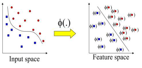
2.3 Kalman Filter
2.4 Discrete Wavelet Transfrom (DWT)
III. Methodology
IV. Results and Discussions
V. Conclusions


References Reducing Support Vector Machine Classification Error by Implementing Kalman Filter
- Ming Ge, R. Du, Cuicai Zhang, Yangsheng Xu, “Fault diagnosis using support vector machine with an application in sheet metal stamping operations”. Mechanical Systems and Signal Processing 18, 2004, pp. 143-159.
- D. Isa, R. Rajkumar, KC Woo, “Pipeline Defect Detection Using Support Vector Machine”, 6th WSEAS International conference on circuits,systems, electronics, control and signal processing, Cairo, Egypy, Dec 2007. pp.162-168.
- M. Hassan, R. Rajkumar, D. Isa, and R. Arelhi “Kalman Filter as a Pre-processing technique to improve Support Vector Machine”, Sustainable Utilization and Development in Engineering and Technology (STUDENT), 2011, Oct 2011, DOI: 10.1109/STUDENT.2011.6089335.
- Rajpoot, K.M, and Rajpoot, N.M, “Wavelets and support vector machines for texture classification”, Multitopic Conference, 2004. Proceeding of INMIC 2004, 8th International, pp.328-333.
- Lee, Kyungmi and Estivill-Castro, Vladamir, “Support vector machine classification of ultrasonic shaft inspection data using discrete wavelet transform”, Proceddings of the International Conference on Machine Learning, MLMTA’04, 2004.
- Sandeep Chaplot, L.M. Patnaik, and N.R. Jagannathan, “Classification of magnetic resonance brain images using wavelets as input to support vector machine and neural network”, Biomedical Signal Processing Control 1, (2006), pp.86-92.
- Lozev, M. G., Smith, R. W. and Grimmett, B. B., “Evaluation of Methods for Detecting and Monitoring of Corrosion Damage in Risers”, Journal of Pressure Vessel Technology. Transactions of the ASME, Vol. 127, 2005.
- Anonymous (2009, April 1)“Gazprom reduces gas supplies by 40% to Balkans after pipeline rupture”, [Online]. Available: www.chinaview.cn.
- Lebsack, S.,“Non-invasive inspection method for unpiggable pipeline sections”, Pipeline & Gas Journal, 59, 2002.
- Demma A., Cawley P., Lowe M., Roosenbrand A. G., Pavlakovic B., “The reflection of guided waves from notches in pipes: A guide for interpreting corrosion measurements”, NDT & E International. Vol. 37, Issue 3, 167-180. Elsevier, 2004.
- Wassink and Engel, Applus RTD Rotterdam, The Netherland, (2008, April 8), “Comparison of Guided waves inspection and alternative strategies for inspection of insulated pipelines”, Guided Wave Seminar, Italian Association of Non-destructive Monitoring and diagnostics (AIPnD).Available:www.aipnd.it/onde-guidate/GWseminar.htm.
- Anonymous “Teletest Focus Goes Permanent”, Plan Integrity Limited, Available: www.plantintegrity.co.uk
- Dino Isa, Rajprasad Rajkumar, “Pipeline defect prediction using long range ultrasonic testing and intelligent processing” Malaysian International NDT Conference and Exhibition, MINDTCE 09, Kuala Lumpur, July 2009.
- Rizzo, P., Bartoli, I., Marzani, A. and Lanza di Scalea, F.,“Defect Classification in Pipes by Neural Networks Using Multiple Guided Ultrasonic Wave Features Extracted After Wavelet Processing”, ASME Journal of Pressure Vessel Technology. Special Issue on NDE of Pipeline Structures, 127(3), 2005, pp. 294-303.
- Cau F., Fanni A., Montisci A., Testoni P. and Usai M., “Artificial Neural Network for Non-Destructive evaluation with Ultrasonic waves in not Accessible Pipes”, In: Industry Applications Conference, 2005. Fortieth IAS Annual Meeting, Vol. 1, 2005, 685-692.
- Wang, C.H., Rose, L.R.F., “Wave reflection and transmission in beams containing delamination and inhomogeneity”. J. Sound Vib. 264, 2003, pp.851–872.
- K.L. Chin and M. Veidt, “Pattern recognition of guided waves for damage evaluation in bars”, Pattern Recognition Letters 30 , 2009, pp.321–330.
- V. Vapnik. The Nature of Statistical Learning Theory, 2nd edition, Springer, 1999.
- Klaus-Robert Müller, Sebastian Mika, Gunnar Rätsch, Koji Tsuda, and Bernhard Schölkopf, “An Introduction To Kernel-Based Learning Algorithms”, IEEE Transactions On Neural Networks, Vol. 12, No. 2, March 2001 181
- Burges, Christopher J.C. “A Tutorial on Support Vector Machines for Pattern Recognition”.Bell Laboratories, Lucent Technologies. Data Mining and Knowledge Discovery, 1998.
- Haykin, Simon. “Neural Networks. A Comprehensive Foundation”, 2nd Edition, Prentice Hall, 1999
- Gunn, Steve. “Support Vector Machines for Classification and Regression”, University of Southampton ISIS, 1998, [Online] Available: http://www.ecs.soton.ac.uk/~srg/publications/pdf/SVM.pdf.
- Law, Martin. “A simple Introduction to Support Vector Machines”, Lecture for CSE 802, Department of Computer Science and Engineering, Michigan State University. Available: www.cse.msu.edu/~lawhiu/intro_SVM_new.ppt.
- Kecman, Vojislav, “Support Vector machines Basics”, School Of Engineering, Report 616, The University of Auckland, 2004.
- Sweeney, N., “Air-to-air missile vector scoring”, Control Applicationcs (CCA), IEEE Control Systems Society, 2011 Multi-Conference on Systems and Controls, 2011, pp. 579-586.
- Gipson, J., 2012, ‘Air-to-air missile enhanced scoring with Kalman smoothing’, Master Thesis, Air Force Institute of Technlogy, Wright-Patterson Air Force Base, Ohio.
- Gaylor, D.E, 2003, ‘Integrated GPS/INS Navigation System Design for Autoomous Spacecraft Rendezvous’, Phd Thesis, The University of Tezas, Austin.
- Huang, Shian-Chang, “Combining Extended Kalman Filters and Support Vector Machines for Online Price Forecasting”, Advances in Intteligent System Research, Proceedings of the 9th Joint Conference on Information Sciences (JCIS), 2006.
- Lucie Daubigney and Oliver Pietquin, “Single-trial P300 detection with Kalman Filtering and SVMs”, ESANN 2011 Proceeding, European Symposium on Artificial Neural Networks, Computational Intelligence and Machine Learning, 2011.
- Welch G. and Bishop G., 2006, “An introduction to the Kalman Filter”, Department of Computer Science, University of North Carolina, viewed.
- Grewal M.S. and Andrews A.P., 2001, Kalman Filtering: Theory and Practice Using MATLAB, 2nd Edition, A Wiley-Interscience Publication, New York.
- Shoudong Huang, “Understanding Extended Kalman Filter – Part II: Multidimensional Kalman Filter” March 2009, [Online] Available: http://services.eng.uts.edu.au/~sdhuang/Kalman%20Filter_Shoudong.pdf
- Mallat, S. A Wavelet Tour of Signal Processing, 1999, Elsevier.
- Anonymous “Discrete Wavelet Transform”, Available: www.plant http://en.wikipedia.org/wiki/Discrete_wavelet_transformintegrity.co.uk.
- Lee, K. and Estivill-Castro, V., Classification of ultrasonic shaft inspection data using discrete wavelet transform. In: Proceedings of the Third IASTED International Conferences on Artificial Intelligence and application, ACTA Press. pp. 673-678.
- Lin C.J, Hong S.J, and Lee C.Y, “Using least squares support vector machines for adaptive communication channel equalization”, International Journal of Applied Science and Engineering, 2005, Vol.3, pp.51-59.
- Sebald, D.J.and Bucklew, J.A., “Support Vector Machine Techniques for Nonlinear Equalization”, IEEE Transaction of Signal Processing, Vol. 48, No.11, 2000, pp.3217-3226.
