Регистрация параметров верхней атмосферы Восточной Сибири при помощи интерферометра Фабри-Перо KEO Scintific «Arinae»

Spectrophotometric studies of night airglow are one of the main instruments for studying Earth’s upper at mosphere [Shefov et al., 2006]. Features of the generation of optical radiation in the upper atmosphere, namely its spectral lines and vertical stratification of airglow for certain wavelengths, provide information on motion and temperature of air masses in various atmospheric layers. A physical phenomenon that makes it possible to determine atmospheric gas velocity and temperature is the Doppler shift of the wavelength of recorded radiation, which arises from collective (wind) or chaotic (temperature) motion of radiating particles. Using well-known expressions (for example [Landau, Lifshitz, 1988])

AX = pF X_o V mcc

(X о is the wavelength of immobile emitting matter, Xs is the central wavelength of the registered spectral line, AX is the recorded widening of the spectral line, v, T, m are the velocity, temperature, and mass of luminous matter particles, k is the Boltzmann constant, c is the speed of light in vacuum), we can estimate the sensitivity necessary for the successful application of the method:

5X = Xo-Xc =^, c

5AX = AX ₂ -AX 1 = X _o

In order for the instrument to record changes in wind velocity at 10 m/s and temperature at 10 K for a wavelength of 630 nm, its sensitivity should be such that an investigator can observe changes of position and width of the spectral line at 10–5 and 10–4 nm respectively.

One of the currently available methods for recording the spectral composition of optical radiation with this sensitivity is a method for observing interference in parallel rays in the Fabry–Perot interferometer [Born, Wolf 1973]. There are many scientific instruments (for example, [Wu et al., 2004; Shiokawa et al., 2012; Anderson et al., 2009; Ignatiev et al., 1998]) that use this method to study optical airglow. The field of view of these instruments, except for that described in [Anderson et al., 2009], is units of degrees, so in a single observation session we can obtain characteristics of only a certain local region of the celestial sphere. Therefore, to extend functionalities, some of these instruments scan the celestial sphere with an automated periscope as an input window. Interferometers record observations with CCD cameras, which allow one to store an entire interference pattern in digital form and to process measurements after an observation session. A key issue in observations at this sensitivity level is the stability of parameters of an observation system. Modern Fabry–Perot interferometers for observing Earth’s upper atmosphere are equipped with temperature stabilization systems and laser calibration light sources adopted to monitor stability of their operation.

We de a l with one of such instrum e nts installed i n the Geophysical Observatory (GO) of th e Institute of S olarTerrestrial Physics SB RAS (the vill a ge of Tory, 52° N, 103° E). We describe its design and a data proc e ssing method. Diurnal variations in some c h aracteristics o f the upper atm o sphere, obtained with the interferomet er , are given and c ompared to similar param e ters recorde d with other instruments. A comparison is m ade with up p er atmosphere p arameters obtained by mo d els NRLMSI S E-00 [Picone et a l., 2002] and HWM14 [Dr o b et al., 2015]. We have used observational data acquired at ISTP SB RAS GO from J u ne 2016 to February 2017.

INTERFEROMETER DESIGN

The Fabry–Perot interferometer installed in GO is manufactured by KEO Scientific (Canada) and is called KEO Scientific Arinae. A detailed description of its design is given in [Shiokawa et al., 2012]. We present only some distinctive features essential for our study. The schematic of the tool is shown in Figure 1 (left). One of the main specific systems of the instrument is the periscope consisting of two mirrors, which can independently rotate in perpendicular planes with the aid of step motors (Figure 1, right). The step motors are controlled automatically, thereby providing the opportunity to adaptively manage the observation process and to aim the periscope to any point in the celestial sphere. After the input window, the radiation passes through a passband filter 70 mm in diameter. The diameter of the filter determines the diameter of the pupil of the aperture of the instrument. The interferometer is equipped with a set of six equal-sized filters with a passband of ~1 nm each and central wavelengths of the passband of 630.0, 557.7, 427.8, 589.3, 732.0, and 843.0 nm. The filters are placed in a filter wheel cassette. Like the input window, the filter wheel cassette is controlled by a step motor with the ability to automatically control and change the filters according to a preset program. The cassette is equipped with a temperature stabilization system that automatically maintains the desired constant temperature of the filters. After the filter, the light flux comes to the Fabry–Perot etalon, made in the form of two circular reflecting surfaces 70 mm in diameter with an air gap 15 mm high.

The air gap is hermetically sealed off fr o m the environ m ent. The reflecting surfac e s are made o f a material with a low c oefficient o f thermal expansion (0± 0 .007·10^–6 K ^{– 1} in a range 0–50 °C) an d are coated with a specialize d reflective c o mposition o p timized for wor k ing with ra d iation at w a velengths o f 630.0 and 557.7 nm (the r e flection coe f ficient is 0. 7 –0.9). The plate surface qual i ty is λ /100. T he interferen c e pattern is

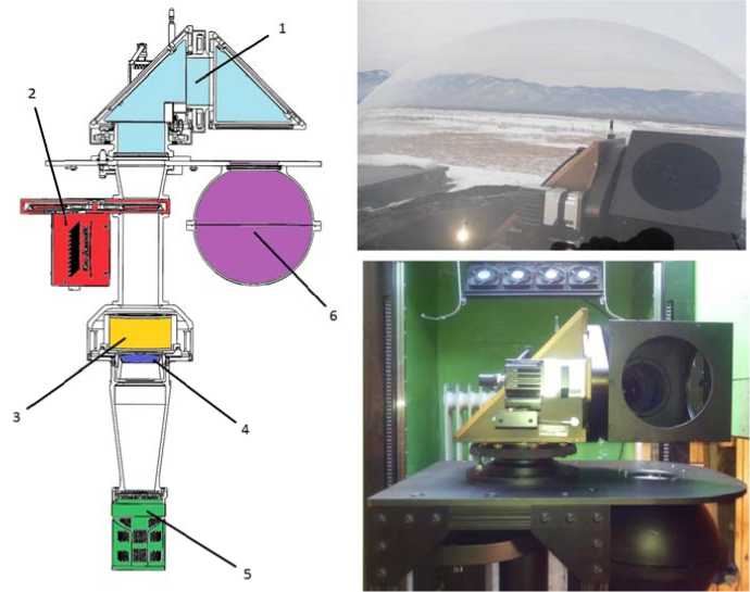
Figure 1 . General scheme and photog r aphs of the int e rferometer per i scope: 1 is the periscope; 2 is the filter whee l cassette; 3 is the Fabry–P e rot etalon; 4 is the focusing l e ns; 5 is the CC D camera; 6 is the calibration l ight-scattering sphere. The in p ut window is oriented suc h that the interferometer can re c ord a helium- n eon laser light scattered in the sphere

wheel cassette, has a temperature stabilization system that automatically maintains temperature required for operation. The interference pattern, formed on the lower plate of the etalon, is focused by the collecting lens on the CCD matrix. The focal length is about 30 cm; the size of the matrix is 1.3×1.3 cm2. Thus, the field of view of the instrument is ~2.5°. This instrument uses a PIXIS 1024B CCD camera. Resolution of the CCD matrix is 1024×1024 pixels; to reduce noise, the matrix is cooled to the operating temperature of –70 °C, using a Peltier element. At this stage of the study, the said resolution is not required; therefore, to reduce costs for processing information coming from the camera and increase the sensitivity, the image from the camera undergoes the so-called binning procedure. The actual resolution decreases to 512×512 pixels. For additional calibration, the interferometer is equipped with a helium-neon laser connected through a light guide to a special lightscattering sphere. The output window of the sphere is attached to the periscope support. The input window can be oriented such that laser light from the scattering sphere would fall on the input window of the interferometer and can automatically calibrate the instrument during measurements. The output of the laser is equipped with an automatically controlled shutter to prevent laser light from entering the input window of the interferometer when observing the celestial sphere. The instrument is controlled by a personal computer connected to the interferometer systems (periscope engines, filter wheel cassette motor, heaters and thermal sensors of filters and etalon, control of the CCD camera shutter, data transmission system, camera temperature stabilization system, and laser shutter control) via specialized interfaces. The personal computer has special software that synchronously controls all the interferometer systems according to a preset program. The interferometer is mounted on an electromechanical elevator in a room with a transparent dome 1 m in diameter.

In t h e room, co n stant positi v e temperatu r e is maintain e d; the dome h as a windsh i eld defog sy s tem to prevent condensatio n . Photos of t he interfero m eter in the wor k room are presented in Fig u re 1, right.

METHOD OF PROCESSING INTERFERENCE

PATTERN AND CONDUCTING OBSERVATION

E xamples of i nterference p atterns (inte r ferograms), for m ed in the interferometer w h en observin g nightglow, and calibration la s er light are s hown in Fig u re 2. There are m any techni q ues that allo w us to determine wind velocity and te m perature fr o m interfere n ce patterns for m ed by the Fa b ry–Perot res o nator (see, f o r example,

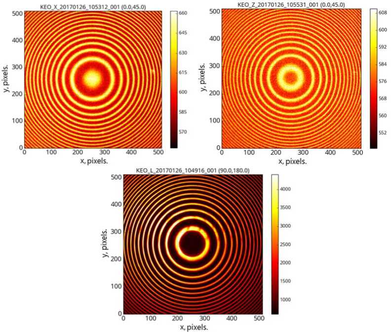
Figure 2 . Interferograms obtained fr o m observation of nightglow a t a wavelengt h of 630.0 nm ( top left) and 557.7 nm (top right). At th e bottom is an interferogram f rom observati o n of the heliu m -neon laser li g ht (632.8 nm).. The color int e nsity scale is in relative u n its

[Ignatyev, Yugov, 1995]); however, the use of twodimensional CCD matrices for recording interference patterns and the computational capabilities of modern computers open up somewhat greater possibilities of image processing. Therefore, the basis for processing observational data is the method described in [Harding et al., 2014]. Its application requires us to represent a two-dimensional interferogram as one-dimensional through circular integration of the available twodimensional dataset, using the method described in [Makela et al., 2011]. As a result, the two-dimensional interferogram is represented as one-dimensional, reflecting the dependence of intensity on distance, which is measured from the center of the interference pattern. For successful circular integration of the interferograms obtained from airglow observation (especially under variable intensity of recorded light), we should periodically register calibration laser interferograms. These calibration data help to determine current parameters of the measuring system, such as the center of the interference pattern and the instrumental function. The instrumental function, which, in fact, is a modified Airy function [Borne, Wolff, 1973], contains additional information on inhomogeneities of the optical system of the interferometer. Hereinafter, we utilize this instrumental function to describe interferograms obtained from nightglow observations. This model is an integral function composed of a set of modified Airy functions entering the integral with values of intensity and wavelength corresponding to an assumed form of spectral line of detected light. Obviously, the determination of parameters of the instrumental function and the model function describing a recorded signal requires performing the procedure of “fitting” the model functions to experimental data. For this purpose, we use least-squares minimization with the Le-venberg–Marquardt algorithm [Marquardt, 1963].

Harding et al. [2014] logically present moments of reduction of the Airy function describing the interference pattern from monochromatic radiation at the output of the ideal Fabry — Perot etalon to a modified form; therefore, it makes no sense to dwell on these operations here. We give only the final result and describe some modifications essential for this study. The modified Airy function has the form

rm

A ( r , X ) = J b ( 5 , r ) A ( 5 , X ) ds + B , (5) 0

where X is the radiation wavelength, r is the distance from the center of the interference pattern, r m is the radius of the boundary of the interference pattern. In fact, (5) is the convolution of the Airy function, which has a variable intensity depending on r , necessary to take into account vignetting of the optical system,

I 0

A ( s , X ) =

4R sin2

(1 - R )2

2 n nt

----cos a s

X

with a kernel reflecting defects of the optical system, which blur the image on the matrix, b (s, r) =

1 [ ( s - r ) ² , exp^ 2 , _x 2 no ² ( r ) о ⁽ r )

plus a background B , which naturally arises from thermal noises of pixels and penetration of the background radiation, uniformly distributed over wavelengths, through the input filter and etalon.

In the above expressions, R is the reflection coefficient of the Fabry — Perot etalon’s surfaces, n is the refractive index of the medium between the reflecting surfaces of the etalon, t is the distance between the etalon’s surfaces, α is the magnification factor; I 0 , I 1 , I 2 are constant coefficients.

The dependence of the Gaussian kernel width on the distance in the CCD matrix is as follows:

^o( r ) =

where о ₀, a 1 , o ₂ are constant coefficients.

Expression (5) in [Harding et al., 2014] is used as an instrumental function. By minimizing the difference of this model with one-dimensional laser interferograms, we can find current values of the constant coefficients in (6)–(8), reflection coefficient, gap of the etalon, and magnification factor. The values derived from the minimization are used as nonvarying parameters in the model of night-sky interferograms:

X2 __

S(r)=J A(r, X)Y(X)dX + B,                   (9)

X 1

where Y ( X ) reflects the shape of the spectral line:

Y ( X ) = Y ₀ + Y exp <

1 f X-X _c ] 2 ( AX )

Integration limits in (9) are chosen based on characteristics of the input filter. The values reflecting the background B , line intensity 1 ₀, its position X _s and width AX are determined by minimizing the difference between observed data and the model of night-sky interferograms. After minimizing (9) with night-sky observations, X s and AX obtained from (1) and (2) determine temperature and velocity of the emitting medium along the line of sight of the interferometer.

To improve the stability of the interferogram processing method put forward in [Harding et al., 2014], we modify the expressions describing interference patterns. The following changes in models of calibration laser light and airglow can be considered essential:

• 1)    substituting the polynomial dependence of intensity (the numerator in (6)) by the first terms of the Fourier expansion such that this dependence looks like expression for Gaussian kernel width (8);

• 2)    replacing the magnification factor α by the direct calculation of the inclination angle of input radiation

registered in a certain coordinate of t he CCD ma t rix r : α r= arctg( r / F );

• 3)    introducing the squared relati o nship betwe e n the background and the distance on the C CD matrix B = B 0 + B 1 r ²;

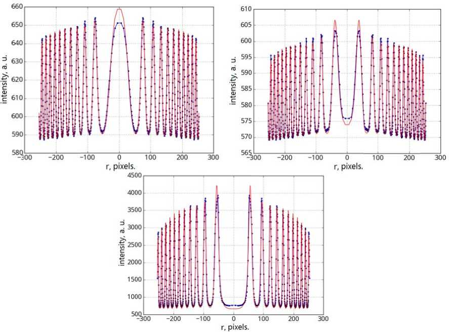
• 4)    symmetric expansion of a o n e-dimension a l interferogra m into the negative scale r .

The last operation doubles the n u mber of poi n ts in the existin g dataset. At first glance, this leads onl y to a useless inc r ease in the computational time for mini m ization. How e ver, we think that this app r oach is valid since it facilitates more stable operation o f the minimi z ation algorithm. In particular, it automatically meets the natural require m ent of the zero derivative for the inten s ity at the center of an interference pattern. Examples o f one-

VvVvW

8VVVv

3000 i^soo c 2000

-"300    -200    -100      0      100     200     300

r, pixels.

-100     0      100

r, pixels. 4500

5 595

™ 590 o'

5 585

— 580

= 630

s' 620

§ 610

200     300

-300    -200

-200    -100      0      100     200     300

r, pixels.

Figure 3 . One-dimensional interfero g rams (blue cu r ves) and functions with sele c ted parameter s describing th e se interferograms (red c urves). Interferograms deriv e d from observ a tion of the ni g htglow at a w a velength of 6 3 0.0 nm (top l e ft) and 557.7 nm (top right). At the bottom is an interfe r ogram obtaine d from observation of helium-neon laser ligh t (632.8 nm)

The mentioned capability of the interferometer to automatically change the direction of observation along with the assumption of a certain time of medium stationarity in an observed region determines the method of wind velocity measurements. Suppose that at heights corresponding to the maximum intensity of atomic oxygen airglow in a region with a characteristic size of several hundreds of kilometers the wind blows in the same direction for 15 minutes. Then, if during this time we perform observations in the north, south, west, and east directions at an angle to the horizon, the obtained interferograms would be formed by radiation whose wavelength is shifted by some value depending on the direction of observation. This shift is caused by the so-called dimensional interferograms and results of minimization of the models to the observational data used in this paper are given in Figure 3. As seen below, despite some deviations of the resulting model functions from experimental data, the reliability of the obtained upper atmosphere parameters is at an acceptable level.

It s h ould be note d that the inte r ferogram dat a processing methods and mini m ization proc e dures are per f ormed using the P ython langua g e [van Ross um , 1995], as w ell as packages Mahotas [ C oelho, 2013] for image p r ocessing to for m one-dimensi o nal interfero gr ams and Lm f it [Newville et a l ., 2014] to i m plement pr o cedures for fi tting model func t ions to obser v ational result s .

line-of-sight velo c ity – the pro j ection of the wind velocity o n the direct i on of obser v ation, comb i ned with a possible systemat i c shift arisi ng from inacc u racy of the mo d el describing the interfero g ram. Becaus e of the station a rity of the w i nd velocity du ring a series of observation s in different directions, t h e estimated l ine-of-sight velocities are rigi d ly bound (Fi g ure 4):

L N = L0 + H sin 0 + V cos 0,(11)

LS = L0 + H sin 0-V cos 0,(12)

LE = L0 + H sin 0 + U cos 0,(13)

LW = L 0 + H sin 0-U cos 0,(14)

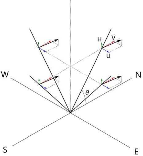
Figure 4. Directions of observations and projection of wind velocity. The black arrow is the full wind velocity, the green arrow is the vertical wind velocity, the red and blue arrows are meridional and zonal components of the horizontal wind velocity where LN, LS, LE, LW are line-of-sight velocities in the directions to the north, south, east, and west respectively; L0 is the possible systematic shift due to inaccuracy of the model describing the interferogram; H is the vertical wind velocity; U, V are zonal and meridional components of the horizontal wind velocity; 0 is the elevation angle of observation. Expressions (11)–(14) show that to derive values of the zonal and meridional wind, we should subtract line-of-sight velocities of opposite directions:

L N - L S = 2V cos 0 ,                           (15)

L E - L W = 2U cos 0 .                          (16)

This operat i on also eliminates the possible systemati c error in the meas u ring system and the vertica l wind effect.

Tempe r ature as a scalar quantity does not req u ire a change of direction to be estimated. Of course, there also may b e some systematic errors i n this param e ter in the model, but, unfortunately, a cha n ge in directi o ns in this case c a nnot eliminate them beca u se the statio n arity of temper a ture in time in the observ e d region do e s not imply the absence of spatial tem p erature gra d ients. Therefore, there are no special requir e ments for te m perature mea s urements, except for the s ufficient ex p osure time to for m an interference pattern.

Thus, t h e sequence of nighttime o bservations l ooks like a set o f directions changing with time (see Ta b le).

Typical interferograms for the said exposure times have already been presented in Figures 2, 3. Figure 5 shows variations in the I0 line intensity, background optical radiation near the 630 nm emission B0, horizontal wind temperature and speed for the night of January 26–27, 2017, obtained with the described method of Sequence of nighttime observations performed with the inter- ferometer

Direction Wavelength Exposition North 630.0 120 s North 557.7 60 s East 630.0 120 s East 557.7 60 s South 630.0 120 s South 557.7 60 s West 630.0 120 s West 557.7 60 s zenith 630.0 120 s zenith 557.7 60 s laser 630.0 30 s observation and processing of the results. We have chosen January 26, 2017 because at this very night in particular observation hours there were abnormally low temperatures (~200–300 K) estimated from the 630 nm emission (T630). Note here that the minimum monthly averages of T630 for winter months are ~400–450 K; for summer months, ~600–750 K. The maximum values of T630 are recorded in twilight periods of observations: ~800–900 K for summer and ~700 K for winter. Figure 6 demonstrates the behavior of the parameters of the instrumental function model, which are the most critical for measuring wind velocity (the product of the thickness of the gap of the etalon and the refractive index nt, the focal length F), and temperature (reflection coefficient of the etalon’s surfaces R and the width of the Gaussian kernel describing image blurring S0). These parameters were obtained from periodic calibration of the tool during the night. The lack of agreement in the behavior of constants of the instrument and characteristics of the recorded light suggests that the model is most likely to be valid and can be used for follow-up studies.

T he behavior of the recor d ed intensity of airglow, tem p erature, and wind is con s idered belo w . Here, we wan t to discuss t h e behavior o f the backgr o und optical radi a tion. As see n , in the sec o nd half of t h e night for mos t analyzed di r ections the m ean backgro u nd value is hig h er and its var i ations are co n siderable. T h is is due to the p resence of an additional l ight source w ith a wide spectrum in the f i eld of view o f the tool. S u ch an addition a l source of light in this s pectral range can be the airg l ow continuu m , light from stars, planets, the Moon, and other natura l and artific i al sources. I f there are clou d s in the interferometer fi e ld of view, t he intensity of t h is additiona l light sourc e will increa s e and vary con s iderably wit h time. Thus, the paramet e r B ₀ can be use d to indirectl y estimate th e presence o f cloudiness duri n g observations. In this c a se, the beh a vior of this para m eter means that from th e beginning of the observati o n session on January 26, 2017 at ~18 : 00, the sky was clear, and cl o uds gathered at ~00:00 on January 27, 201 7 . This is confirmed by ph o tos taken b y wide-angle surveillance cameras installed n earby the int e rferometer. Des p ite the app e arance of c l oudiness, th e degree of clou d cover is su c h that it prac t ically does n o t affect the beh a vior of the o b served inten s ity. It is imp o ssible to

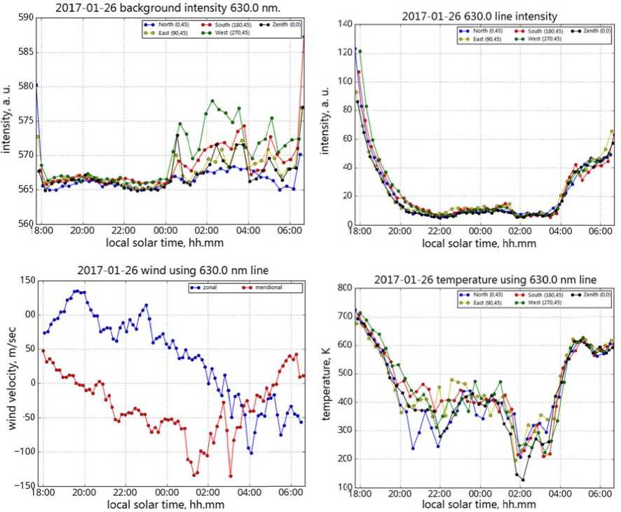
Figure 5 . Background intensity (top left), line inten s ity (top right), zonal and meridional wind v e losities (posit i ve directions of wind vel o city to the north and east) ( b ottom left), t e mperature (bo t tom right), as observed in t he atomic oxyg e n airglow at 630.0 nm during the night on January 26–27, 2017. Colo r indicates dat a for different o b servation dire c tions

say that there is no cloudiness effect on the esti m ated wind velo c ity and direction. The ra d iation scatte r ed in the cloud l ayer and recorded in a c e rtain directi o n results from mixing of radiation com i ng from dif f erent directions a bove the cloud layer. Thi s can seriousl y distort wind d ata. In the same way, the observed te m perature could be affected by the light scattering, b u t the recorded significant temperature decrease (the in t erval from 01:3 0 to 03:30 on January 27, 2017) does no t synchronize with the occurrence of cloudiness.

In addition, it should be noted t hat cloud sc a ttering would lead to the observed in c rease in te mp erature since the emission of lines, shifted due t o the presence o f wind in different direct i ons, “mix” i n the clouds, thereby broadening the observed line.

In the immediate vicinity of t h e interfero m eter, there are a number of optical inst r uments det e cting airglow. Next, we compare some observation r e sults obtained with the interferometer to d ata acquire d with an all-sky camera operating at a w a velength of 6 30.0 nm, with a spectrometer recording 630.0 and 5 57.7 nm atomi c oxygen intensities, and with an in f rared spectrometer recording hydroxyl emission ( (6-2) band, 834.0 nm) in the mesopause r e gion.

NIGHT VARIATIONS OF INTENSITY AS OBTAINED WITH THE INTERFEROMETER, AND COMPARISON WITH

SPECTROPHOTOMETER DATA

Night variatio n s in intensit i es of 630 a n d 557.7 nm ato m ic oxygen e m issions are shown in Fi g ure 7. The win t er period is taken here b e cause the ti m e span of obs e rvations duri n g this seaso n is maximu m . Intensity vari a tions in the 6 30.0 nm lin e features an evening decrease associated with sunset, a slight midni g ht increase caused by an increase in the el e ctron densit y at a height of emission [Aka s ofu, Chapm a n, 1974], an d a morning incr e ase due to s u nrise. Verti c al lines indicate the momen t s of sunset and sunrise f or a height of 250 km abo v e the interfe r ometer and a t the magn e toconjugate point. The dusk e m ission at 63 0 nm may be, to a greater extent, due to th e photodissoc i ation of mo l ecular oxygen in the Schuman–Runge co n tinuum; in t h e night period, the 630 nm emission is r elated to dis s ociative recombination with O⁺ 2 , NO⁺ io n s; and at pre- d awn hours, a n o table contrib u tion to the 6 30 nm emission can be made by photoelectrons from m agnetoconju g ate regions [Se m enov, 1975; K rassovsky e t al., 1976; T o roshelidze,

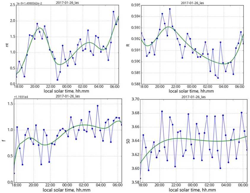
Figure 6 . Product of the gap between the etalon an d the refractive index (meters) (top left); refl e ction coeffici e nt of the etalon’s surfaces (top right); focal length (in CCD matrix p ixels) (bottom left); width of the Gaussian k ernel blurring t he image (in matrix pixels) (bottom right). The green line indicates s m oothed data used in the mode l of night-sky i n terferograms

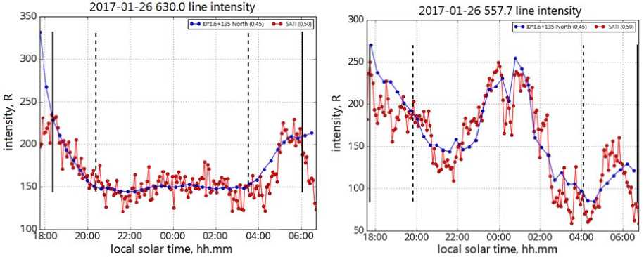
Figure 7 . Night variations in the 630.0 nm emissio n intensity as d erived from interferometer ( b lue) and spect r ophotometer (red) data (l e ft); night variations in the 557.7 nm emissi o n intensity as derived from i n terferometer ( b lue) and spect r ophotometer (red) data. V ertical lines are sunset and s u nrise at 250 a n d 90 km abov e the interfero m eter (solid lin e s) and at the m agnetoconjugated point (dashed lines)

1991, Kononov, Tashchilin, 2001]. The height of the maximum atomic oxygen emission of 557.7 nm (~97 km) being much lower than that of 630 nm (~250 km), the times of local sunrise and sunset for 97 km are at the boundary of the observation interval. An observable characteristic feature of the night variation in the green line intensity in winter is the midnight maximum (Fish- kova, 1983), which arises from tidal activity. Figure 7 shows night variations in the 630 and 557.7 nm emission intensities as derived from data from the SATI-1 spectrophotometer [] placed near the interferometer.

Interferomete r data are ta k en for the r e gion of the sky closest to the spectrophoto m eter field of view.

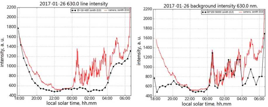
Figure 8 . Night variations in the 630. 0 nm line inte n sity as inferred from data obt a ined with the i nterferometer (black curve) and the all-sky camera (red curve); night variations in th e backgroun d intensity for t h e 630.0 nm li n e as derived f rom data acquired with t he interferometer (black curve) and integral intensity from the all-sky ca m era (red curve )

Night vari a tions in the intensity of emissions d e rived from data o btained with various instr u ments are in good agreement ; hence the nightglow int e nsity seems to be correctly r e presented in the interferogram model. A t this stage, using spectrophotometer data, we can perf o rm a simple cal i bration of the intensity recorded by the interferometer, assuming a linear relatio n ship betwee n the incoming l i ght flux and the relative u n its of the int e rferometer int e nsity. For the green line, t h e correction coefficient is 4 ; for the red line, in additio n to the multi p licative part, 1 .6, there is an additive c o mponent eq u al to 135. This may be due to the presen c e of an addi t ional background for the 630.0 nm line.

We have compared interferometer data to data obtained with a wide-angle camera equipped with a 630.0 nm filter []. By comparison, in the images captured by the camera we select areas corresponding to the interferometer field of view. The behavior of the integrated intensity, recorded in these areas of the images, is shown in Figure 8. It is appropriate here to compare the results obtained with the camera to the behavior of not only the intensity of the red line, but also of the background, since the line and background intensities are not separated in the wide-angle camera in this case. The simultaneous observation with the camera and interferometer shows that a fairly good agreement of recorded intensities occurs in the absence of cloudiness (from the beginning of observations till midnight, see above), while in the presence of cloudiness (from midnight to the end of observations) a better agreement is observed between the integrated intensity recorded with the camera and the background recorded with the interferometer.

NIGHT VARIATIONS

IN TEMPERATURE FROM

THE 630.0 nm LINE AND PROBLEM OF LOW TEMPERATURES

Temperature variations as observed in the 630.0 nm line overnight are mainly as expected (Figure 9). There is an evening decrease and a morning increase in tem- perature caused by sunset and sunrise. As shown by neutral atmosphere models and observational data [Fisher et al., 2015], the maximum variation in the gas-kinetic temperature at a height of around 250 km overnight is about 150 K. The night variations in Doppler temperature T630 ~ 400–500 K observed in this case differ significantly from the NRLMSISE-00 model data. The values of T630 calculated from the empirical model [Shefov et al., 2007] for the night of January 26, 2017, vary from ~750 K at the beginning of the night and to ~514 K in the pre-dawn hours around the local midnight, thus being also much higher than the temperature measured with the interferometer.

Note a rapid, about one ho ur, decreas e in the observ e d Doppler t e mperature b y about 200 K at 02:00. Such a signific a nt temperat u re decrease cannot be caused by variations in para m eters of the observation syst e m since the behavior of t he paramete r s R and S 0 (Figures 5, 6) does not correlat e with the be h avior of the obs e rved tempera t ure.

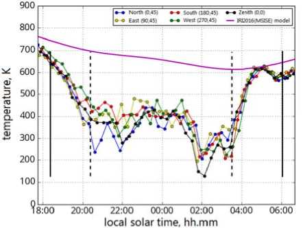
Figure 9 . Night v ariations in te m perature from the 630.0 nm line and NRLMSI S E-00 data. R e d, blue, green, and yellow curves are temperat u re values for d ifferent directions of observation; the purple c urve indicates model data. B lack vertical lines denote sunset a nd sunrise ab o ve the interfer o meter (solid) and a t the magnetoc o njugate point ( dashed lines)

Another factor capable of causing the temperature to fall to such abnormally low values may be the presence of a spurious signal, for example, the hydroxyl emission in the (9-3) band, which overlaps the wavelength of 630.0 nm. As shown in [Hernandez, 1974], such a hypothetical possibility exists.

It should be noted that Nakamura et al. [2017] report the results from determination of temperature from the 630 nm line and show that the temperature values obtained with the Fabry — Perot interferometer are periodically much lower than the atmosphere temperature at the height of the emission layer. The authors explain this problem of underestimation of the measured temperature by distortion of a signal, recorded with the interferometer, owing to the hydroxyl emission ((9-3) band) at a wavelength that almost coincides with the 630 nm atomic oxygen emission. Thus, other scientific teams also face the problem of systematic underestimation of temperature from interferometric measurements; therefore, it calls for further investigation. Some pilot studies of this problem can be carried out using instruments of GO Tory, which is equipped with a Fabry — Perot interferometer and a spectrometer, which allows us to examine variations in the hydroxyl emission intensity.

Let us examine in more detail several interferograms obtained during the night on January 26–27, 2017 at 18:00, 00:00, and 02:00 local solar time (Figure 10). As the 630.0 line intensity decreases, the second ring system becomes more pronounced in a one-dimensional interference pattern. It is not visible in two-dimensional interferograms due to a very noisy signal. If we construct model one-dimensional interferograms for wavelengths corresponding to the hydroxyl emission lines P 1 (2) 628.75, P 2 (3) 629.79, and P 1 (3) 630.7 nm [Hernandez, 1974] in one plot with experimental data, we can compare the second ring system with one of these lines. Figure 11 shows two interferograms for 18:00 and 02:00 local solar time. Experimental data, the most well-chosen model, and the model with wavelengths corresponding to hydroxyl emission and exact position of the oxygen line ³ P ₂–¹ D ₂ 630.0 308 nm are plotted in different colors [Hernandez, 1974]. In this case, we need the model for the exact value of the oxygen line because there can be some constant systematic shift in the observation system at the accuracy level considered. Therefore, to identify the second line, we should shift all model curves of hydroxyl and oxygen ring systems to the right by the same amount to fit the model curves describing the oxygen ring system with observational data. Here the hydroxyl line P 1 (3) will coincide with the second ring system. According to [Hernandez, 1974], this line is the brightest in this triplet. This agrees with observations we perform. Thus, the data presented in Figure 11 suggest that with a significant decrease in the intensity of the oxygen line ³ P 2 – ¹ D 2 , the hydroxyl line P 1 (3) begins to resolve, but due to minimization the model still describes the brightest oxygen line. Hence, the temperature derived from minimization is in fact the temperature obtained from observation of the 630.0 nm line.

As already noted, the presence of cloudiness can distort parameters of observed optical radiation and thus can distort estimated wind and temperature characteristics. A considerable temperature decrease, by more than 100 K, occurred almost immediately after sunset, and an additional decrease to ~150 K began at 02:00. This does not correlate with the observed cloud behavior. Moreover, the lowest temperature at this night was recorded at the zenith, while the maximum background intensity hypothetically capable of distorting the results was observed westward.

Figure 12 shows variations in the intensity of the hydroxyl emission arising at mesopause heights ((62) band, ~ 87 km), and in ionospheric parameters: electron density at the ionization maximum N m F2 and the height of the ionization maximum H m F2 versus direction-averaged intensity and Doppler temperature for the 630.0 nm line. The observations were made with an infrared spectrometer located in the immediate vicinity [Medvedeva et al., 2012] and with a DPS-4 ionosonde. The data are given for January 26, 2017. We can say that the behavior of the 630 nm line intensity correlates with the Doppler temperature behavior. This is especially noticeable during temperature anomaly. The behavior of the hydroxyl emission intensity anticorrelates with the behavior of the observed temperature, but this anticorrelation can in some cases be delayed for some time, and in some cases may be absent (Figure 13), despite the abnormally low temperature. It should be noted that the temperature behavior during the anomaly on January 26, 2017 is in good agreement with the behavior of the charged component of the upper atmosphere (Figure 12, right).

This event is of special interest and will be considered in detail in follow-up studies.

NIGHT VARIATIONS

IN TEMPERATURE FROM

THE 557.7 nm LINE.

CALIBRATION PROBLEM. COMPARING WITH DATA ON ROTATIONAL TEMPERATURE OF HYDROXYL MOLECULES

It is unreasonable to use a helium-neon laser for calibration with the 557.7 nm light filter because a signal in this case is extremely weak. The model parameter which greatly depends on emission wavelength and is of key importance in determining temperature is the reflection coefficient R . To work in the green spectral region, we received a laboratory-measured wavelength dependence of the reflection coefficient of the etalon’s surfac-esfrom manufacturers of the interferometer. This dependence was used to scale this parameter in the instrumental function while minimizing for data obtained at a wavelength of 557.7 nm. Night variations in temperature as observed in the green line of atomic oxygen for two different nights are shown in Figure 14. The absolute temperature as derived from the interferometer

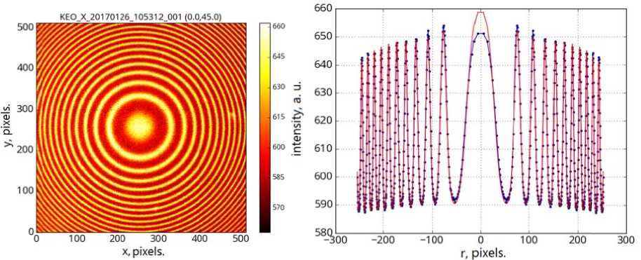
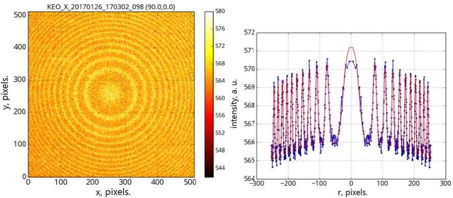
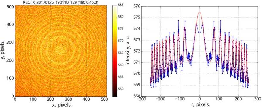
Figure 1 0 . Two-dimensional interfer o grams obtaine d at 18:00, 00:00, and 02:00 local solar tim e (left, from to p to bottom). One-dimen s ional interferograms obtaine d in the same p eriods (right, from top to b o ttom). Blue c u rves indicate o bservational data; the re d curve, the model selected fro m the observat i onal data

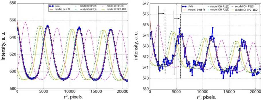
Figure 1 1 . A part of the interferogra m for 18:00 lo c al solar time ( l eft). The blue curve indicate s observational data; the red one is the model selected from the observational data, t he yellow cur v e is the mode l selected fro m the observati o nal data, but with a wav e length of 630.0308 nm. Dash e d curves are m odels selecte d from the obse r vational data, b ut with wavelengths corresponding to the three nearest hydroxyl e m ission lines a s derived from data obtained i n [Hernandez, 1974]. Arrow s and vertical lines show t h e direction and value of the shift needed to a ccount for the systematic bia s in the observ a tion results

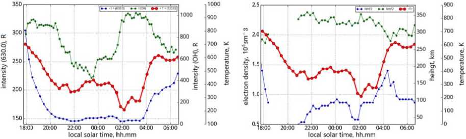
Figure 1 2 . Behavior of Doppler tem p erature (left, r e d curve) and i ntensity (left, b lue curve) fro m the 630.0 nm line for the night of Jan u ary 26–27, 2017. Green colo r marks variati o ns in the hydr o xyl emission i ntensity, the ( 6 -2) band. Tem p erature variations (right, red curve) from the 630.0 n m line and va r iations in ionospheric param e ters: the heig h t of the F2-la y er maximum (green curve) and electron density at the F 2-layer maxi mu m (blue curv e )

data turned out to be much higher th a n expected d ue to the insuffi c ient accuracy of R , theref o re the Figur e s use a scaled value.

To approximately calibrate interf e rometric te m perature meas u rements, we can use data on rotational temperature o f hydroxyl molecule obta i ned from sp e ctral observatio n s of OH molecule emissi o n ((6-2) ban d , 834

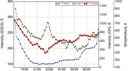
Figure 1 3 . Variations in the Doppler te m perature (red c urves) and intensity (blue curves) from the 63 0 .0 nm line. Gr e en curves are hydroxyl e m ission intensity variations (6-2). Variations for t he night of Jan u ary 2, 2017, w h en there was d e layed anticorre l ation between the Doppler temperature of the 630 nm line a nd the hydrox y l emission intensity (left). Vari a tions for the ni g ht of January 21, 2017, when there was no anticorrelation between the Do p pler temperatu r e of the 630 n m line and the hydroxyl emissio n intensity (6-2)

nm) with the infr a red spectro m eter located i n the immediate vicinity [Medvedeva et al. 2012]. T h e hydroxyl emission layer in t ensity is ma x imum at a h e ight of ~87 km a nd is ~9 km t hick; the rot a tional tempe r ature of the OH molecule corresponds to th e atmosphe r ic temperature at the emissi o n height [Sh e fov et al., 20 0 6].

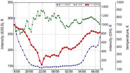
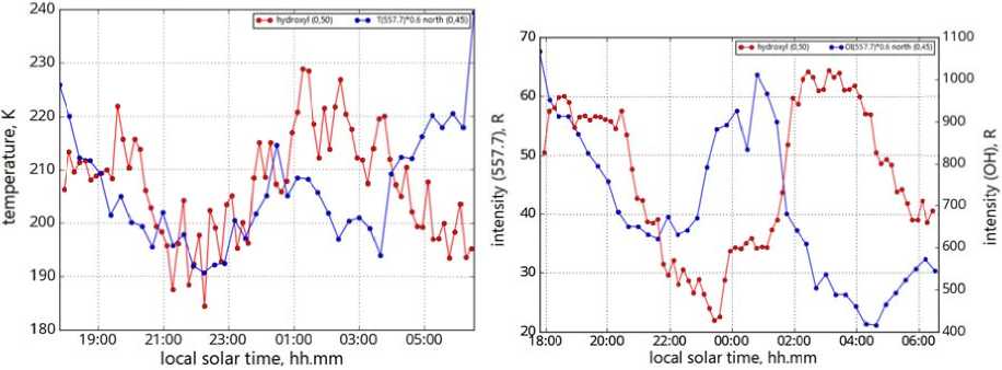
Figure 1 4 . Night variations in tempe r ature obtained from observations of OH e m ission (6-2) (r e d curve) and g reen oxygen line (blue curve) (left). Night variations i n OH emission i ntensity (6-2) ( red curve) and green oxygen l ine (blue curv e ) for January 26, 2017 (right)

Since the m aximum atomic oxygen e m ission at 557 . 7 nm (~97 km) i s relatively close to the hei g ht of the max i mum hydroxyl e m ission (~87 km), we can compare the temperature values and, in some approximation, dete r mine the correction coefficient for the tem p erature deter m ined from inter f erometric observations of t h e 557.7 nm emission. To fi t the observed temperature s , we use a c o rrection coefficient of 0.6 for the interferometer data . It is evident that for two nights the use of t h is coefficient gives good agre e ment of temperature variat i ons approxi m ately till 00:00, after which the temperature values ob t ained from obse rv ations of hydroxyl and at o mic oxygen emissions begin to differ. A possible reaso n for this ma y be a change in wind conditions at 90–10 0 km. As sho w n in Figure 15, it is at this time that the w i nd parameter s , obtained usin g the green oxygen line, ch a nge.

NIGHT VARIATIONS IN WIND AS DERIVED FROM 630.0AND 557.7 nm EMISSION DATA

557.7 and 630.0 n m lines are s hown in Figure 15. The Fig u re also prese n ts wind vari a tions obtain e d generally con s istent with m o del data.

Absolute win d velocity an d characteristic times reflecting maximu m and mini m um daily w ind values roughly coincide. The differe n ces seem to arise from pec u liarities of u p per atmosph e re condition s and condition s of observati o ns on a part i cular day. W a ve activity, specific geomag n etic conditi o ns, transfer of energy stor e d in the tro p osphere fro m the bottom up, clouds, and other factors , ignored in t he HWM14 model, can sign i ficantly dist o rt the wind p attern. Furt h ermore, the mo d el HWM14 d i sregards sol ar activity, he n ce there are sign i ficant differ e nces in win d amplitude. In order to correctly compar e wind charac t eristics obtai n ed with the interferometer to HWM14 mo d el data, foll o w-up studies s hould average observed c h aracteristics or consider specific conditio n s of the up p er atmosph e re in input para m eters of the model.

Wind direction and velocity deter m ined from b o th

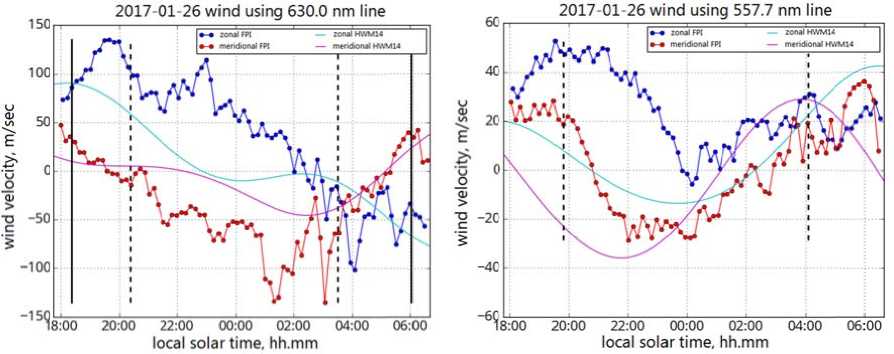
Figure 1 5 . Night variations in zonal a n d meridional w inds (left), o b tained from observations of t h e red oxygen l ine (blue and red curves) on January 26, 2017. On the right is the sam e for the green oxygen line. Blue and violet c urves are zon a l and meridional winds from the HWM14 model

CONCLUSIONS

A new instrument designed to determine spectral characteristics of optical airglow at middle latitudes has been put into operation. We have carried out observations of characteristics of the spectral oxygen lines with wavelengths of 557.7 and 630 nm. Using the obtained characteristics, we have determined the behavior of line and background intensities overnight, as well as the behavior of temperature and wind velocity for different heights in Earth’s atmosphere. We have compared the results to data obtained with other instruments and to model outputs.

We have analyzed some factors and geophysical conditions that potentially affect the accuracy of measurements. In particular, we have shown that for the night of January 26, 2017 considered, the hydroxyl emission ((9-3) band), whose lines fall into the passband of the 630 nm interference filter, could not have a significant effect on the determination of the temperature T 630 . During some nights, there is characteristic anticorrelation between the behavior of hydroxyl emission intensity ((6-2) band) and temperature T 630 , which could be an additional factor exhibiting the effect of hydroxyl signal on estimated temperature. However, this anticorrelation is often delayed (of order of half an hour), and in some cases, at a significant decrease in T 630 , there is no anticorrelation. These facts may suggest that the relationship between the observed temperature T 630 and the hydroxyl emission intensity is formed by processes occurring in the upper atmosphere, and is not an error in observation or processing of the results.

We have noted the nature and degree of influence of the background emission caused by atmospheric scattered radiation background from external natural sources. We have compared 557.7 and 630 nm emission intensities, temperature (557.7 nm emission) with data from the all-sky camera in the 630 nm emission, the SATI-1 spectrometer (557.7 and 630 nm emission spectrometer), and the infrared spectrometer (rotational OH temperature ((6-2) band). We have calculated and reported model values (NRLMSISE-00, HWM14) of kinetic temperatures and winds for heights of the maximum 557.7 and 630 nm emission at the site of the Fabry — Perot interferometer observation. A fairly good agreement has been obtained for model and experimentally observed values of wind velocity, whereas temperatures T₆₃₀ in some intervals significantly differ from model values. The closest agreement between temperatures is observed in the pre-dusk hours. The most acute and still unresolved issue in these results is the observed extremely low (~ 200 K) temperatures (in the period 01:30–03:30 LT), determined from the 630 nm emission. In this interval, a sufficiently high correlation of T 630 with f 0 F2, related to the 630 nm line emission region, does not allow us to unambiguously associate this result with the inaccuracy in the interferometric technique of determining T 630 or with the influence of meteorological conditions; it requires additional experimental and theoretical studies and, possibly, refinement of the technique for processing interferometric observations.

Note that a possible explanation for the observed extremely low temperatures, comparable to the tempera- tures at heights of the upper mesosphere–lower thermosphere in the 557.7 nm emission region (~85–115 km), could be one of the known channels of population of the 1D atomic oxygen level associated with the 557.7 nm emission at the transition from 1S to 1D. In this case, each emission of 557.7 nm photon produces one excited O(1D) atom With hypothetical extreme decreases in the 630 nm emission intensity from the ionospheric F2 region formed by dissociative recombination, a certain contribution to the height-integral 630 nm emission intensity (and hence to the temperature) could also be made by the emission from this wavelength from the 557.7 nm emission height. However, it is generally accepted that, because of the long lifetime of the metastable level 1D and high rates of its collisional deactivation at these heights, there is no 630 nm emission at the upper mesosphere–lower thermosphere heights. The relationship between kinetic temperatures obtained with atmospheric models and Doppler temperatures obtained from interferometric observations in the 630 nm emission will be examined more thoroughly in follow-up studies.

The comparison between the temperature obtained from observations of the OH emission (6-2) and that obtained from observations of the 557.7 nm oxygen line shows a significant discrepancy between these characteristics, despite the fact that the emission sources are vertically spaced by about 10 km. So, it is unacceptable to use hydroxyl emission to calibrate the interferometer that records emission at 557.7 nm. Therefore, for the 557.7 nm line, we should search for additional means of calibration of the instrument. In this case, it may be reasonable to use a low-pressure mercury lamp, which has a line in the green spectral region, as a source of line optical radiation.

In general, the results obtained with the Fabry — Perot interferometer designed to observe the airglow in two atomic oxygen lines of 557.7 and 630.0 nm demonstrate validity of this instrument and its quite high potential for follow-up studies of thermodynamic mesosphere– lower thermosphere characteristics.

We have used data from the Fabry — Perot interferometer included in the optical complex of the Angara Multiaccess Center.

The work was financially supported by the project “Study of dynamic processes in the neutral atmosphere– ionosphere–magnetosphere system” (unique number 03442014-0006) and grant No. NSH-6894.2016.5 of the President of the Russian Federation for State Support of Leading Scientific Schools.