Removing Noise from Speech Signals Using Different Approaches of Artificial Neural Networks

Author: Omaima N. A. AL-Allaf
Journal: International Journal of Information Technology and Computer Science(IJITCS) @ijitcs
Article in issue: 7 Vol. 7, 2015.
Free access
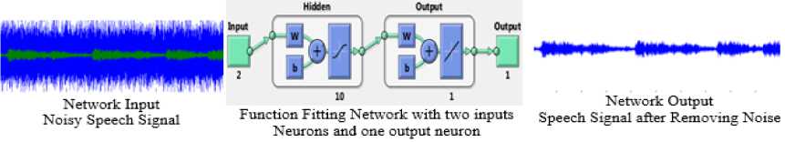
In this research, four ANN models: Function Fitting (FitNet), Nonlinear AutoRegressive (NARX), Recurrent (RNNs), and Cascaded-ForwardNet were constructed and trained separately to become a filter to remove noise from any speech signal. Each model consists of input, hidden and output layers. Two neurons in the input layer that represent speech signal and its associated noise. The output layer includes one neuron that represent the enhanced signal after removing noise. The four models were trained separately on stereo (noisy and clean) audio signals to produce the clean signal. Experiments were conducted for each model separately with different: architecture; optimization training algorithms; and learning parameters to identify model with best results of removing noise from speech signal. From experiments, best results were obtained from FitNet and NARAX models respectively. TrainLM is the best training algorithm in this case. Finally, the results showed that the suggested architecture of the four models have filtering ability to remove noise form both trained and not trained speech signals samples.
Signal Enhancement, Artificial Neural Networks, Function Fitting (FitNet), Nonlinear AutoRegressive (NARX), Recurrent (RNNs), and Cascaded-ForwardNet
Short address: https://sciup.org/15012318
IDR: 15012318
Text of the scientific article Removing Noise from Speech Signals Using Different Approaches of Artificial Neural Networks
Published Online June 2015 in MECS
Artificial Neural Networks (ANNs) includes many neurons that operate in parallel and connected via weights [1]. ANNs have been used largely in the fields of image and signal processing [2]. Many ANN models that differ in architecture and training algorithms were suggested in the past. Multi-layer perceptron and backpropagation neural network (BPNN) are largely used ANN models. These models require large number of iterations for training network on any specified problem. Many literature approaches have been carried out to improve the speed up the network learning [3][4][28..32]. The nonlinear ANN nature and ability to learn from their environments in supervised and unsupervised ways make them highly suited for solving difficult signal processing problems. But all these available techniques have certain limitations.
Signal enhancement is process of performing nonlinear filtering of a signal for noise reduction. Is critical to understand the nature of problem formulation when dealing with signal processing applications, so that the most ANN approaches can be applied. Recently, ANNs are found to be a very efficient tool for signal enhancement. It is important to assess the impact of ANN on the performance, robustness, and cost-effectiveness of signal processing systems.
Another important issue is how to evaluate ANN approaches, learning algorithms, and structures for solving signal processing problems [5].
ANNs may provide a new approach for signal filtering. Recent experimental suggests that ANNs may be able to reduce noise for many applications [6]. There are few literature researches adopted different ANNs models for removing noise from signal. At the same time, the filtering ability of ANN architectures of most of these literature studies were limited to training set signals. These literature approaches were not able to remove noise from untrained signals or filtered the noise with bad quality and generate the signal with some noise. Other literature studies required long time for training process.
Therefore, we need ANN approaches and models for signal enhancement that remove noise from any speech signal. Also, we need ANN models that generate high values of Peak Signal to Noise Ratio (PSNR) and less values of Mean Square Error (MSE). We need to reduce the time required for the training process.
In this research, four ANN models were constructed and implemented (in MathLab 2013a) for signal enhancement system: Function Fitting (FitNet), Nonlinear Autoregressive (NARX), Recurrent (RNNs), and Cascaded-ForwardNet to improve the speed of convergence and enhance the signals by obtaining high PSNR, MSE and best values of R2 (coefficient of determination of a linear regression). Three optimization algorithms were used in training process (LM, GD, and GDM). Many experiments were conducted to determine the ANN model with its architecture that lead to less learning time and best performance. Comparisons between the four models were conducted also. The research is organized as follows: section II includes related literature and section III describes signal enhancement. Section IV includes details about ANN used models. Section V includes research methodology. Section VI includes experiments and finally section VII concludes this work.
-
II. Related Literature
Many literature studies for noise reduction from speech signal were based on different approaches. Other literature studies were based on ANN for signal enhancement each with different model and architecture. The goal is to define a model that give best results for signal enhancement. At the beginning, Kevin, 1988 [6] explored BPNN approach to filtering noise from signals. Experiments were conducted using single sine wave inputs, multiple sine wave inputs, and human speech inputs. The networks' outputs were then compared to the original signals to determine the network's performance. But network's filtering ability was strictly limited to signals from the training set. The networks were not able to generalize enough to filter signals whose frequencies had never been encountered.
Speech enhancement is concerned with neural processing of noisy speech to improve the quality of speech signal. Tlucak, 1999 [7] described ANNs approaches for speech enhancement. He described an experiment with implementation of two channel adaptive noise remover via direct time domain mapping approach.
Whereas, Badri, 2010 [8] used BPNN and Recurrent ANN (RNN) for noise reduction to enhance the captured noisy signals. They presented the effect of training algorithms and network architecture on ANN performance for a given application. The PSNR was not calculated to determine the enhanced signal. Whereas the minimum obtained MSE is 0.0112. Adaptive filtering technique is one of digital signal processing areas and used in noise cancellation. Noise cancellation is a common and necessary in today telecommunication systems. The LMS algorithm is one of the most efficient criteria for determining the values of adaptive noise cancellation coefficients but it suffers slow convergence rate under low Signal-to-Noise ratio (SNR). Therefore, Miry, et. al., 2011 [9] presented an adaptive noise canceller algorithm based fuzzy and neural network for noise canceling problem of long distance communication channel. Whereas, Pankaj and Anil, 2012 [10] reviewed some speech enhancement techniques to remove noise from speech. They concluded that the fuzzy and neural algorithms used for minimizing noise from a set of sound files. The Root Mean Square Error (RMSE) and number of epochs are less and at the same time the membership functions are also less.
While, Debananda, et, al., 2012 [11] discussed the use of BPNN for noise filtering to remove noise from a noise signal with implications for the signal processing. Thus research lack of discussion related to experimental results such as PSNR and RMSE .
And, Chatterjee, et, al., 2013 [12] presented BPNN as an adaptive filtering technique for removing noise from ECG signal using the Recursive Least Square (RLC) method. They extracted 12 significant features from an echocardiogram (ECG) dataset. ECG signal is obtained after carrying out noise cancellation followed by Recursive Least Square method filtered.
Finally, Andrew, et, al., 2012 [13] introduced recurrent auto encoder ANN to remove noise from input signal for automatic speech recognition (ASR). They trained the model on noisy and clean audio signals to output clean signal. The model makes no assumptions about how noise affects signal, nor the existence of noise environments.
The results of literature related to noise enhancement showed that the performance of recently suggested ANN models and approaches to enhance the untrained signal is low against the signals used in training process. At the same time most of the recently suggested models in literature studies require long time for training process. Thus, we need ANN model for signal enhancement that leads to: less ANN training time; less MSE and highest values for PSNR.
-
III. Signal Enhancement
Signal enhancement is plays an important role in many applications. There are many literature researches for removing the noise from the signal. All these available techniques have certain limitations. Speech enhancement techniques tend to reduce or remove the noise from speech signal. Different types of speech enhancement systems using a single microphone have been proposed and tested. All of these systems are based on techniques which recover the clean speech signal by enhancing the Signal to Noise Ratio (SNR). The performances depend on type of noise and the information they require about noise. It should be noted that the increase of SNR will improve the quality of the speech signal [14]. There are four types of speech enhancement methods:
-
A. Filtering
Adaptive filtering techniques like Kalman filtering have been used for speech enhancement [15]. The Kalman filter yields an optimal solution to the adaptive filtering problem based on LMSE. Unless the noise is stationary and perfectly known that must be done iteratively [16]. According to changing of noise over a time period and overlapping of frequencies of noise and signal, the Adaptive filtering become important. The ability of adaptive filters to operate satisfactorily in unknown and time-varying environments without user intervention and improving their performance during operation by learning statistical characteristics from current signal observations has made them more efficient [12].
-
B. Noise subtraction
The noise and speech are assumed to be uncorrelated and additive. The power spectrum of cleaned speech is obtained by subtracting the noise power spectrum from the spectrum of noisy speech [17]. The method assumes that the noise varies slowly so that the noise estimation obtained during a pause can be used for suppression.
-
C. Space Mapping
Speech enhancement is a process of transforming noisy speech into clean speech by mapping. For instance, spectral mapping has been implemented by a set of rules obtained by vector quantization techniques. It is possible to implement arbitrarily complex space transformations thanks to connectionist ANNs. Even multi-layer perceptrons have been trained on learning samples to realize a mapping of noisy signals to noise-free speech which has been tested with success in an auditory preference test with human listeners [18].
-
D. Hidden Markov Models (HMM)
Decomposition is a method which makes it possible to separate speech from additive noise [19]. It is assumed that speech and noise are both modeled by separate HMMs and that noisy speech corresponds to a composition model combining these two models. This method is rather computationally demanding, but it has been demonstrated to perform satisfactorily even in bad SNR conditions.
-
IV. Neural Networks Models
Fig.1 shows Multilayer feed-forward ANNs that consist of neurons arranged in layers with only forward connections to units in subsequent layers [20]. The connections have weights associated with them. The input layer units distribute the inputs to units in subsequent layers. In the following layers, each unit sums its inputs and adds a bias to the sum and nonlinearly transforms the sum to produce an output. This nonlinear transformation is called the activation function of unit [5].
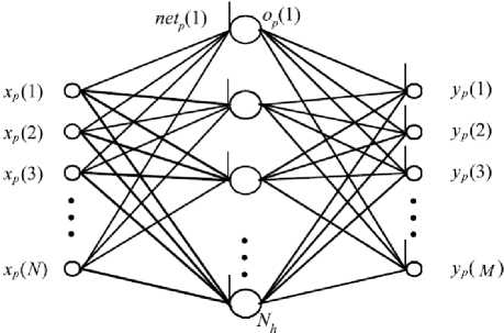
Fig. 1. Multilayer feed-forward ANN [20]
The output layer units have linear activations. The training data set consists of Nν training patterns {( x p, t p)}, where p is the pattern number. The input vector x p and desired output vector t p have N and M dimensions.
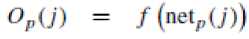
y p is network output vector for pth pattern. The thresholds are handled by augmenting input vector with an element x p (N + 1) and it is equal 1. For the jth hidden unit, the net input net p (j) and output activation Op(j) for pth training pattern are shown in (1) and (2) [1][3][5].
v+l netp(J) = 52 w^’ *’> ' xp^' 1 -j -Nh
where w(j, i) denotes the weight connecting the ith input unit to the j th hidden unit. For MLP networks, a typical sigmoid activation function f is shown in (3) [1][3][5].
/(^0)) =
For trigonometric networks [23], the activations are Sines and Cosines. The kth output for the pth training pattern is y pk and is given by (4) [1][3][5]:
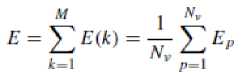
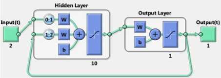
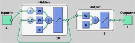
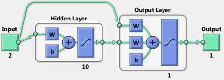
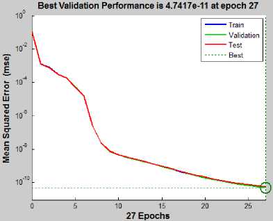
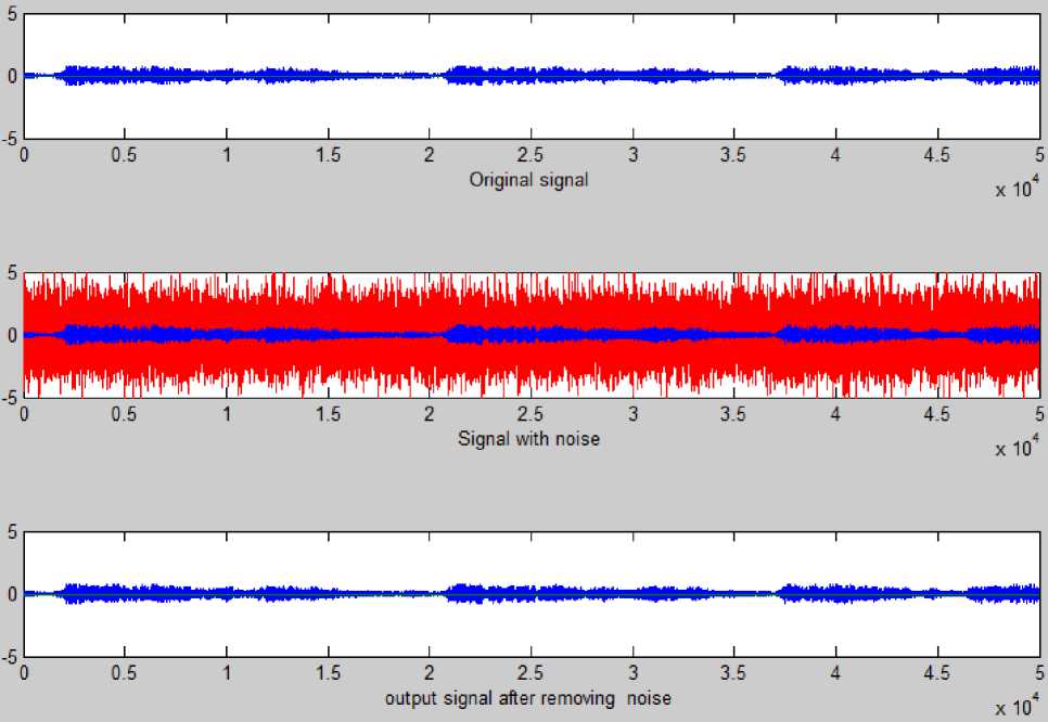
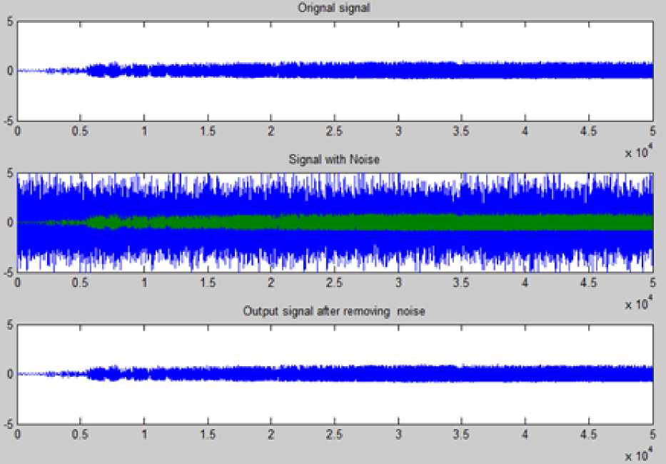
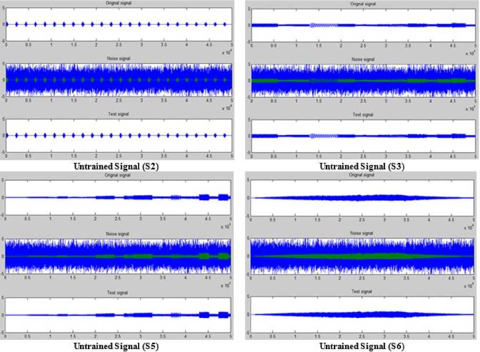
ЛГ+1 Nh yph = 52 ш^к-^■ хр^+52who Where wio(k, i) denotes the output weight connecting the ith input unit to the kth output unit and who(k, j ) denotes the output weight connecting the j th hidden unit to the kth output unit. The mapping error for the pth pattern is calculated using (5) [1][3][5]. Ep = У2 Dp* ~ ?p*] Where tpk denotes the kth element of pth desired output vector. In order to train ANN in batch mode, the mapping error for kth output unit is defined as (6) [1][3][5]. The overall performance of ANN an be measured as MSE and written as (7) [1][3][5]: Then, the adjustment of ANN weights to minimize the error between network’s prediction and actual output. This is to adjust weights values when ANN gaining extra knowledge after each iteration. Output ypk is compared with target output Tpk using (8) [1][3][5]: δk = (Tpk – ypk) ypk (1- ypk) (8) For every neuron in hidden layer, the error term is calculated using (9) [1][3][5]: δpk = ypk (1- ypk) Σδpkwpk (9) Where δpk is error of output layer and wpk is weight between hidden and output layer. The error is propagated backward from output layer to input layer to update weight of connections using (10) [1][3][5]: wjk(t+1)=wjk(t)+ ηδk yk + α(wjk(t)–wjk(t–1)) (10) Both of η: learning rate and α: momentum factor are specified at the start of training and determine speed and stability of ANN [1][3][5]. A. Function Fitting ANN The FitNet is a type of feed forward networks, which are used to fit an input output mapping relationship. A FitNet with one hidden layer and enough neurons [21][22]. The output is calculated directly from the input through FitNet connections like BPNN and Cascade BPNN. The number of connections between each two layers in ANN is calculated by multiplying total number of neurons of the two layers, then adding number of bias neurons connections of the second layer. Fig.2 shows architecture of noise removal from speech signal based on system FitNet model. Fig. 2. The Architecture of Signal Enhancement System Based on Function Fitting ANN B. Nonlinear Auto-Regressive eXogenous (NARX) NARX is a nonlinear autoregressive model which has exogenous inputs in time series modeling. The NARX is a recurrent dynamic network with feedback connections enclosing several layers of network. The model relates the current value of a time series which one would like to explain or predict to both: past values of the same series; and also current and past values of the driving (exogenous) series. That is, of the externally determined series that influences the series of interest. The model contains: error term which relates to the fact that knowledge of the other terms will not enable the current value of the time series to be predicted exactly. Such a model can be stated algebraically as shown in (11) [23]. ^ yt-1, y, - 2, У, -3V, V u,, u-1, u,-2 , u,-3 , * + £, Here y is the variable of interest, and u is the externally determined variable. Information about u helps predict y, as do previous values of y itself. Here ε is the error term (noise). For example, y may be air temperature at noon, and u may be the day of the year (day-number within year). The function F is some nonlinear function (polynomial). F can be ANN, a wavelet network, or a sigmoid network [23]. Although dynamic networks (time serious) can be trained using the same gradient-based algorithms (BP) that are used for static networks, the performance of the algorithms on dynamic networks can be quite different, and the gradient must be computed in a more complex way [21][22][24]. Fig.3 shows the architecture of NARX model that was conducted in this research. Fig. 3. NARX Architecture C. Recurrent Neural Network (RNN) ANNs can learn dynamic or time-series relationships. In dynamic networks, the output depends not only on the current input to network, but also on current or previous inputs, outputs, or states of network [21][22][23][24]. RNN is a neural network that operates in time. At each time step, it accepts an input vector, updates its hidden state via non-linear activation functions, and uses it to make a prediction of its output. RNNs form a rich model class because their hidden state can store information as high-dimensional distributed representations and their nonlinear dynamics can implement rich and powerful computations, allowing the RNN to perform modeling and prediction tasks for sequences with highly complex structure [25][26]. Fig.4 shows the architecture of RNN model that conducted in this research. Fig. 4. Recurrent NN (layrecnet) Architecture D. Cascaded Forward Neural Networks These are similar to feed forward networks such as BPNN with exception that they have a weight connection from the input and every previous layer to the following layers. Fig.5 shows the architecture of Cascaded-ForwardNet model that was conducted in this research and has connections from layer 1 to layer 2, layer 2 to layer 3, and layer 1 to layer 3. This ANN also has connections from input to all three layers. Fig. 5. Cascaded-ForwardNet Architecture Feed-forward networks with more layers and connection might learn complex relationships more quickly like cascade-forward networks. Additional connections might improve speed at which network learns desired relationship [21..24]. E. Training Algorithms for ANN models The optimization training algorithms adjusted the ANN weights with the goal to minimize the performance function. In static feed forward networks or RNN, the performance function to be minimized is taken to be the MSE, between model-desired output and actual response. In each synapse between connected neurons the training function calculates the output error and determines the adjustments to the network’s weights and bias. There are many training algorithms that can be used for ANN training such as: Gradient descent (GD); Gradient descent with momentum (GDM); Gradient descent momentum and an adaptive learning rate (GDX); Levenberg-Marquardt (LM) and Bayesian regularization (BR). These training algorithms can be used to train any ANN to adjust networks' weights to reduce errors as possible as. V. Research Methodology In this research, four ANN models: FitNet (Fg.2), NARX (Fig.3), RNN (Fig.4), and Cascaded-ForwardNet (Fig.5) were constructed and implemented to remove noise from any signal and obtaining good results of RMSE, PSNR and reducing the training time. Each model was suggested to include 3 layers (input, hidden and output). In this research, three different optimization training algorithms were used to train the four ANN models separately to get best results for noise removing system. These optimization training algorithms are as follows [22]: GD; GDM and LM. The network architecture and parameters are shown in details in Table 1. Whereas, Fig. 2 shows the general view of noise removal system. A. Algorithm of Training Process The main steps of training process of each model are as follows: 1) Initialization of network weights with random numbers in the range [0.001 and 0.009]. 2) Initialization of network parameters (η and α) each with value in the range [0.1 and 0.9] 3) Set iterations to zero. 4) Set Threshold error with 0.0000001. 5) Total_error = zero; 6) iterations -> iterations+1 7) Set i with 0 (where i: signal sequence) 8) Open the file which contains the sound signal (si) to be used in training process and read the signal (si) 9) Apply this sound file to input layer neuron. 10) Initialize target output to be same as input signal. 11) Add noise to this sound signal by applying randomly noise to second input neuron. 12) Calculate the outputs of hidden layer units using (1), (2) and (3). 13) Calculate the outputs of output layer units using (4). 14) Calculate the error(i) of the signal (si)= desired output – actual output using (5) 15) If there is another sound signal to be used in training process, then i=i+1, then go to step8, otherwise, go to step 16. 16) Calculate overall ANN error using (6) and (7). 17) Adjust weights between output and hidden layer units using (8), (9) and (10). 18) Adjust weights between hidden and input layer units (8), (9) and (10). 19) If Total_error <= Threshold_error then stop (the network in trained well). Otherwise (need more training), then go to step 5. B. Testing Process The main steps of testing process of each model are: 1) Open file which contains sound signal to be tested. 2) Apply this sound file to input layer neuron. 3) Add noise to this sound signal by applying randomly noise to second input neuron. 4) Calculate outputs of hidden layer units using (1), (2) and (3). 5) Calculate outputs of output layer units using (4). 6) Calculate the MSE, PSNR of input noisy signal, PSNR of output clean signal and R2. Table 1. Network architecture and parameters Parameter Description Number of layers 3 layers (input, hidden and output) Size of signal sample 50000 Size of noise sample 50000 Number of neurons in input layer 2 input units (One unit for signal and other unit for the noise) Number of neurons in hidden layer 10 hidden units Number of neurons in output layer One output unit that represent the signal after removing noise. Training Algorithms LM, GD, and GDM Training patterns Audio files including music with song from MathLab Library (2013a) VI. Experimental Results In this research, four simulation programs to implement the learning and testing processes of the four ANN models: FitNet (Fg.2), NARX (Fig.3), RNN (Fig.4), and Cascaded-ForwardNet (Fig.5). The MathLab 2013a software was used to write programs of speech signal enhancement system. The training data were taken from MathLab library. Also many other sound files were downloaded from website "Odyssey FX | Wav Sound Effects" and used as testing data. Odyssey FX delivers a great source of wonderful sound effects. The Sample Pack includs70 24-bit 100% royalty free wav sound effects samples, Swishes, sweeps and falls Weird hits and stuttered glitch, Retro noises, bleeps and atmospherics inspired by the early Radiophonic Workshop [27]. Number of iterations, MSE, R2 and PSNR were used to check the performance of the signal enhancement system. PSNR will be calculated between the output clean signal and input noisy signal to verify the quality of signal enhancement system. The efficiency of this system was tested by several speech signals. Each model consists of 3 layers (input layer with 2 neurons, hidden layer with 10 neurons and output layer with one neuron). A. Gradient Descent with Momentum (GDM) The first four experiments were based on training the four models separately using GDM training algorithm. One simulation program for each experiment. Table 2 shows: MSE, PSNR, R2 and the number of iteration required to train each model with GDM algorithm. Table 2. Networks Results with GDM algorithm Gradient Descent with Momentum (GDM) No. of hidden units =10 Model Iterations MSE PSNR R2 NARX 678 0.0027 33.73 0.95 Layrecnet 810 0.0019 33.24 0.95 Cascaded 988 0.0008 32.59 0.93 FitNet 465 0.0006 34.76 0.98 We can note from Table 2 that, best results (smallest number of iterations, high value of PSNR, less MSE) were obtained using the FitNet model. Also the next good results were obtained from using the NARX model. B. Gradient Descent (GD) Algorithm Another four experiments were based on training the four models separately using the GD training algorithm. One simulation program for each experiment. Table 3 shows: MSE, PSNR, R2 and number of iterations required to train each model with GD algorithm. Table 3. Networks Results with GD algorithm Gradient Descent (GD) No. of hidden units =10 Network Iterations MSE PSNR R2 NARX 715 0.0044 33.23 0.95 Layrecnet 835 0.0025 33.11 0.94 Cascaded 1013 0.0019 32.22 0.936 FitNet 473 0.0011 34.25 0.97 We can note from Table 3 that, best results were obtained using FitNet model. The results of experiments related to GDM algorithm are near to results related to experiments related to GD algorithm. C. Levenberg-Marquardt (LM) Algorithm Other four experiments were based on training the four models using LM algorithm. Simulation program for each experiment. Table 4 shows MSE, PSNR of input noisy signal, PSNR of output clean signal, R2 and number of iterations to train each model with LM algorithm. Table 4. Networks Results with LM algorithm Levenberg-Marquardt (LM), No. of hidden units =10 Model Iterat ions PSNR of input noisy signal PSNR Of output clean signal MSE Of output clean signal R2 NARX 623 22.18 34.23 0.0001 0.97 Layrecnet 745 20.77 34.12 0.0002 0.97 Cascaded 932 18.87 33.56 0.0004 0.92 FitNet 413 17.88 35.35 0.00005 0.99 From Table 4, the best values of PSNR were obtained from FitNet model. The values of MSE of all models are small whereas the values of R2 are high. We can note from Table 2, Table 3 and Table 4 that, the Cascaded model requires number of iterations more than the other models to convergence. Whereas FitNet model requires less number of iterations. Also, best values of: number of iterations, PSNR, MSE, R2 were obtained from all models when they were trained using Levenberg-Marquardt (LM). Therefore, PSNR of input noisy signal was computed for each model based on LM algorithm. This is done to determine the models ability to remove noise from speech signals. We can note from Table 4 that, the values of PSNR of output signal is high according to the values of PSNR of the corresponding input noisy signal. Therefore, all the models have the ability to remove noise from any speech signal with small differences between PSNR values. Also the best value of PSNR was obtained from FitNet model. D. Impact of learning rate value In this section, other four experiments were conducted for each one of the four models separately. Each model is trained using LM with 10 hidden units. The four experiments used different values of learning rate such as (0.05, 0.005, 0.0003 and 0.00001). Table 5 shows: number of iterations, MSE, PSNR and R2 for each model for every value of learning rate. Table 5. Different values of learning Rate No. node in hidden=10, Levenberg-Marquardt (LM) Model Iterations MSE PSNR R2 learning rate NARX 623 0.0001 34.23 0.97 0.05 589 0.0003 34.51 0.971 0.005 511 0.0013 34.66 0.976 0.0003 491 0.0010 34.71 0.977 0.00001 RNN 745 0.0002 34.12 0.97 0.05 702 0.0004 34.32 0.975 0.005 678 0.0008 34.55 0.977 0.0003 622 0.0004 34.62 0.979 0.00001 Cascaded 932 0.0004 33.56 0.92 0.05 893 0.0007 33.77 0.927 0.005 845 0.0016 33.87 0.929 0.0003 809 0.0005 33.89 0.934 0.00001 FitNet 413 0.00005 35.35 0.99 0.05 397 0.00002 35.75 0.993 0.005 365 0.00010 35.91 0.994 0.0003 311 0.00001 35.93 0.996 0.00001 We can note from Table 5 that there are no notable differences between the values of MSE, PSNR and R2 for all models when decreasing the value of learning rate. But the number of iterations were decreased when decreasing learning rate. E. The Effect of Hidden Layer Neurons Many other experiments were conducted based on training the four models separately on different number of hidden layer neurons (10, 20 and 30 respectively). Table 6 shows the impact of number of hidden neurons on: number of iterations, MSE, PSNR and R2 factors. We can note from Table 6 that increasing the number of hidden layer neurons for each model will lead to increasing number of iterations. At the same time, there is no big differences in values of MSE, PSNR and R2. F. Impact of MSE At the same time, we can note from all experiments related to all models, that the value of MSE start with large value at the beginning of the training process, then decreased gradually during the training process. According to the value of MSE, the training process will stopped at value of MSE near to 0.0000001. Fig. 6 shows the decreasing in MSE values during the training process. Fig. 6. Learning rate during training significance of figure in caption. G. Results of Testing Process Other 12 experiments were conducted based on testing the four models separately using LM, GDM and GD training algorithms respectively. One simulation program for each experiment. The PSNR is calculated for the output signal after removing the noise form it. Table 7 shows MSE and PSNR of input noisy signal, and PSNR of output clean signal for each one of the four model when trained using LM algorithm. Table 6. Impact of number of hidden neurons learning rate =0.00001, Levenberg-Marquardt (LM) Model Itera tions MSE PSNR R2 Number of hidden neurons NARX 491 0.0010 34.71 0.977 10 523 0.0033 34.75 0.979 20 588 0.0013 34.85 0.989 30 RNN 622 0.0004 34.62 0.979 10 697 0.00022 34.69 0.98 20 734 0.00011 34.79 0.985 30 Cascaded 809 0.0005 33.89 0.934 10 845 0.00053 33.85 0.94 20 892 0.00013 34.12 0.945 30 FitNet 311 0.00001 35.93 0.996 10 398 0.00001 35.96 0.997 20 421 0.00001 36.96 0.998 30 Table 7. Results of Testing (LM algorithm) Model MSE PSNR of input noisy signal PSNR of output signal NARX 0.0007 20.12 33.88 RNN 0.0005 19.25 33.65 Cascaded 0.0004 17.64 32.54 FitNet 0.00007 16.22 34.22 Whereas, Table 8 shows MSE and PSNR of input noisy signal, and PSNR of output clean signal for each one of the four model when trained using GDM algorithm. Table 8. Results of Testing (GDM algorithm) Model MSE PSNR of input noisy signal PSNR of output signal NARX 0.0034 20.12 33.53 RNN 0.0023 19.25 33.11 Cascaded 0.0012 17.64 32.35 FitNet 0.0009 16.22 34.55 And finally, Table 9 shows MSE and PSNR of input noisy signal, and PSNR of output clean signal for each one of the four model when trained using GD algorithm. Table 9. Results of Testing (GD algorithm) Model MSE PSNR of input noisy signal PSNR of output signal NARX 0.0067 20.12 PSNR RNN 0.0051 19.25 33.55 Cascaded 0.0032 17.64 33.42 FitNet 0.0023 16.22 32.47 We can note from Table 7, Table 8 and Table 9 that, the best results were obtained from the FitNet model. Also, we can note that the smallest values of MSE and PSNR of all models (NARX, Layrecnet, Cascaded, and FitNet) were obtained when using the LM training algorithm. Therefore, PSNR of the input noisy signal was calculated for all models based on LM algorithm to determine the models ability to enhance noisy speech signals. From Table 7, Table 8 and Table 9, the PSNR values of output signal is high according to PSNR values of the corresponding input noisy signal. Thus, the four models have the ability to remove noise from any speech signal with small differences between PSNR values. H. Ability to Remove Noise form Untrained Signal The testing process is based on the trained and untrained speech signals. Fig.7 shows the input noisy speech signal which was already used in training process. Fig.7 shows also the trained speech signal after the filtering (removing noise) using FitNet model. Also, the four models were succeeded to filter untrained speech signal (S1) from noise. We can note from Fig.7 that the FitNet model can successfully remove noise any trained speech signal. Untrained speech signal (S1) is used to test the FitNet model that is trained using LM. Fig.8 shows untrained clean signal (S1), noisy signal (S1), and finally clean signal (S1) after removing noise using FitNet model. Other experiments for testing FitNet model based on LM on other 5 untrained speech signals (S2..S6). Fig.9 shows the original signal, noisy signal and its enhanced version of four untrained speech signals (S2, S3, S5 and S6). Fig.9 shows the ability of FitNet model to remove noise from any noisy speech signal. Table 10 shows the MSE, PSNR of input noisy signal and PSNR of output clean signal of the 5 untrained signals. Table 10 shows high values of PSNR and low values of MSE. Table 10. Results of Testing Untrained Speech Signals Network Signal MSE PSNR Of input signal PSNR Of output signal FitNet, LM Algorithms, 10 hidden units S1 0.000081 20.45 34.55 S2 0.000073 21.12 34.24 S3 0.00007 16.22 34.36 S5 0.000077 19.07 34.22 S6 0.000083 20.35 34.37 Fig. 7. Original signal, signal with noise, and signal after filtering for already trained speech signal using FitNet model Fig. 8. Original signal, signal with noise, and signal after filtering for already untrained speech signal (S1) using FitNet model Fig. 9. Shows the original signal, noisy signal and its enhanced version of four untrained speech signals (S2, S3, S5 and S6) (FitNet model) VII. Conclusion In this research, Four ANN models: FitNet (Fg.2), NARX (Fig.3), RNN (Fig.4), and Cascaded-ForwardNet (Fig.5) were constructed with 3 layers (input, hidden and output) for speech signal enhancement to remove noise from any signal. Two neurons in input layer to represent speech signal and its associated noise. The output layer includes one neuron that represent the enhanced signal after removing noise. Different number of hidden neurons were used for each model (10, 20 and 30). Three training algorithms (GD; GDM and LM) were used to train each on of the four models separately to become a filter. The MathLab 2013a software was used to write programs of training and testing the four models for speech signal enhancement system. The four models were trained on many stereo speech signals (noisy and clean) to produce the clean signal of the noisy input signal. The training data were taken from MathLab 2013a. Also other sound files were taken from Odyssey FX | Wav Sound Effects [27] and used as testing data. Many experiments were conducted for training/testing each model separately with different: number of hidden layer neurons, learning rate, and training algorithm to identify model with best results of removing noise from any speech signal. Best results (smallest number of iteration, highest PSNR, lowest MSE) were obtained from FitNet model, then from NARAX models respectively. The experiments shows that, decreasing the learning rate parameter will decrease the number of iterations required to train each model. Experiments shows also that, increasing number of hidden neurons will lead to increase number of iterations for learning process. From experiments, TrainLM is the best training algorithm in all experiments. The worst results obtained from Cascaded model. Finally, from experiments, the suggested filtering approach based on FitNet, NARX , RNN and Cascaded models respectively has the ability to remove noise from speech signal as possible as. This is done according to calculate the PSNR of the input noisy signal (17.88dB) and PSNR of output clean signal (35.35dB) for the FitNet model. Also there is a big difference between the two values (PSNR of input and PSNR of output) for the other models (NARX, RNN, Casdcaded). The four models approved in removing noise from speech signal. The filtering based ANN four approaches was tested on both trained and untrained speech signal. The best values of PSNR of output clean signal were obtained from FitNet model (34.22dB) and NARX (33.88dB) respectively.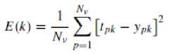
References Removing Noise from Speech Signals Using Different Approaches of Artificial Neural Networks
- R. P. Lippmann. "An Introduction to Computing with Neural Nets," IEEE ASSP Magazine, vol.4, no.2, April 1987, pp.4-22.
- N. K. Ibrahim, R.S.A. Raja Abdullah and M.I. Saripan. "Artificial Neural Network Approach in Radar Target Classification," Journal of Computer Science, vol. 5, no.1, 2009, pp.23-32, ISSN: 1549-3636, Science Publications.
- P. D. Wasserman. Neural Computing: Theory and Practice, Van Nostrand Reinhold Co. New York, USA, 1989, ISBN: 0-442-20743-3.
- Ra´ul Rojas, Neural Networks: A Systematic Introduction, Springer, Berlin Heidelberg NewYork, 1996.
- Yu Hen Huand and Jenq-Neng Hwang, handbook Of Neural Network Signal Processing, Electrical Engineering And Applied Signal Processing (Series), Crc Press Llc, 2002
- Kevin S. Cox, An Analysis Of Noise Reduction Using Back-Propagation Neural Networks, Thesis, Faculty Of The School Of Engineering Of The Air Force Institute Of Technology, Air University, Master of Science In Computer Eng. Captain, Usaf, Afit/Gce/Eng/88d-3, 1988.
- J. TLUCAK, et al, Neural Network Based Speech Enhancement.,Radioengineering. Vol. 8, No. 4, Dec1999.
- Lubna Badri, Development of Neural Networks for Noise Reduction, The International Arab Journal of Information Technology, Vol. 7, No. 3, pp:289-294, July 2010.
- M. Miry, et. al. Adaptive Noise Cancellation for speech Employing Fuzzy and Neural Network, Iraq J. Electrical and Electronic Eng, Vol.7, No.2, 2011, pp: 94-101.
- Pankaj Bactor and Anil Garg, Different Techniques for the Enhancement of the Intelligibility of a Speech Signal, International Journal of Engineering Research and Development,Vol.2, Issue.2, July 2012,pp:57-64, eISSN : 2278-067X, pISSN : 2278-800X, www.ijerd.com
- Debananda Padhi, et, al. Filtering Noises from Speech Signal : A BPNN approach, International Journal of Advanced Research in CS and Software Engineering, Vol.2, Issue.2, Feb2012, ISSN: 2277 128X, www.ijarcsse.com
- Kalyan Chatterjee, et, al. Adaptive Filtering and Compression of Bio- Medical Signals Using Neural Networks, International Journal of Engineering and Advanced Technology (IJEAT),Vol.2 Issue.3, Feb2013, pp:323-327, ISSN: 2249 – 8958.
- Andrew Maas, et, al. Recurrent Neural Networks for Noise Reduction in Robust ASR, INTERSPEECH 2012, 13th Annual Conference of the International Speech Communication Association, Portland, Oregon, USA, September 9-13, 2012. ISCA 2012.
- J.P. HATON, Problems and solutions for noisy speech Recognition, Journal De Physique Iv, Colloque C5, supplement au Journal de Physique 111, Vole 4, May 1994.
- Widrow, B. et, al. Adaptive Noise Cancelling: Principles and Applications, Proc. IEEE, 63(12), pp:1692-1716, 1975.
- Koo, B., Gibson, J.D., Gray, S.D. Filtering of Colored Noise for Speech Enhancement and Coding, International Conference on Acoustics, Speech, and Signal Processing, 1989. ICASSP-89, pp:349-352, Glasgow, 1989.
- Hermansky H. An Efficient Speaker-independent Automatic Speech Recognition by Simulation of Some Properties of Human Auditory Perception, Proc. of: Acoustics, Speech, and Signal Proc., IEEE Int. Conf. on ICASSP '87, Vol.12, DOI:10.1109/ICASSP.1987. 1169803, pp:1159-1 162, Dallas, 1987.
- Tamura, S., Waibel, A.: Noise Reduction using Connectionist Models, Proc. ICASSP-88, 553-556, New York, 1988.
- Varga, A.P., Moore, R.K.: Hidden Markov Model Decomposition of Speech and Noise, Proc. ICASSP-90, 845-848, Albuquerque, 1990.
- C-H Hsieh, M.T. Manry, and H. Chandrasekaran, Near optimal flight load synthesis using Neural Networks, NNSP ’99, IEEE, 1999
- O. De Jesus and M. Hagan, "Backpropagation Algorithms for a Broad Class of Dynamic Networks," IEEE Transactions on Neural Networks, vol.18, No.1, pp.14 -27, Jan.2007.
- MathWorks, Neural Network Toolbox 7.0, MathWorks Announces Release 2010a of the MATLAB and Simulink Product Families, 2010, MathWorks, Inc.
- Wikipedia Encyclopedia 2014,http://en.wikipedia.org /wiki/
- O. De Jesus and M.T. Hagan, "Backpropagation Through Time for a General Class of Recurrent Network," in Proc. of the International Joint Conference on Neural Networks, Washington, DC, vol.4, pp.2638–2643, 2001, ISBN: 0-7803-7044-9, DOI: 10.1109/IJCNN.2001.938786.
- James Martens and Ilya Sutskever, Learning Recurrent Neural Networks with Hessian-Free Optimization, Proceedings of the 28 th International Conference on Machine Learning, Bellevue,WA, USA, 2011.
- Alex. Graves, et, al. A Novel Connectionist System for Improved Unconstrained Handwriting Recognition. IEEE Transactions on Pattern Analysis and Machine Intelligence, vol. 31, no. 5, 2009.
- Odyssey FX | Wav Sound Effects, http://www. wavealchemy.co.uk/odyssey_fx/pid53#purchase, 2014.
- Le Hoang Thai, et al. Image Classification using Support Vector Machine and Artificial Neural Network, I.J. Information Technology and Computer Science, MECS, May2012, 5, pp:32-38, DOI: 10.5815/ijitcs.2012.05.05
- Koushal K. and Gour S. M. T., Advanced Applications of Neural Networks and Artificial Intelligence: A Review, I.J. Information Technology and Computer Science, MECS, Jun2012, 6, pp:57-68, MECS, DOI: 10.5815/ijitcs.2012. 06.08
- Koushal K. and Abhishek, Artificial Neural Networks for Diagnosis of Kidney Stones Disease, I.J. Information Technology and Computer Science, MECS, July2012, 7, 20-25 DOI: 10.5815/ijitcs.2012.07.03
- Debaditya B. and Nirmalya C., A Method of Movie Business Prediction Using Back-propagation Neural Network, I.J. Information Technology and Computer Science, MECS, Oct2012, 11, pp:67-73, DOI: 10.5815/ijitcs.2012.11.09
- Maya L. Pai, et al. Long Range Forecast on South West Monsoon Rainfall using Artificial Neural Networks based on Clustering Approach, I.J. Information Technology and Computer Science, MECS, 07, pp:1-8, June 2014.
