Research on Canal System Operation Based on Controlled Volume Method

Published Online October 2009 in MECS

A canal system can be operated by managing the water volume contained in one or more canal pools, and the volume can be changed to satisfy operational criteria by allowing the pivot point to move within each pool, this is the controlled volume method of operation [1]. The controlled volume method of operation offers the most flexibility of any method of operation. Because a constant depth limitation does not exist, the operational flexibility primarily is restricted by depth fluctuation limits. A canal

Footnotes: 8-point Times New Roman font;

Manuscript received January 1, 2008; revised June 1, 2008; accepted July 1, 2008.

Copyright credit, project number, corresponding author, etc.

system operating by the controlled volume method of operation has the capability to respond to a wide range of flow conditions. Depth fluctuation can be managed to avoid rapid drawdown at the upstream ends of the pools without wasting water or exceeding the maximum depth allowed at the downstream ends. Another aspect might be to transform rapid flow change at the downstream end into a gradual flow change in the upstream canal pools by using pool storage as a buffer, and as a result, the disturbance to the upper pools is minimized.

The controlled volume method of operation requires using the supervisory control method and the complex software developed according to local specific conditions, so this method of operation is most difficult to bring into effect. Although there are many successful engineering examples to adopt the controlled volume method of operation in overseas canal systems [2]–[5], but the control algorithms can only be suitable for their specific operation plans, also there is not detailed data introduction for their concrete methods. Yao et al. [6]-[7] established the operation mode of serial canal system based on the controlled volume method, and the model was successfully tested in the testing canal system proposed by ASCE, but he has not made detailed introduction for specific algorithm to realize the volume control process, also the accurate volume control is not realized. A brief and effective controlled volume algorithm is proposed in the paper on the foundation of predecessors’s studies, and the simulation is carried out to the practical project.

• II.    OPERATIONAL CONTROL MODEL OF CANAL SYSTEM

A. Mathematical Model of Canal System

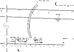
Usually the main canal is divided into canal pools by check gates in series which contains some canalside turnouts. The check gates of upstream and downstream are boundaries of the conjoint pools. The water transfer canal system showed in Fig. 1 is composed of n canal pools, and there is a huge reservoir upstream as water source [1].

G(1)                G(2)

Canal pool 1

G(i)                   G(i+1)

Canal pool i

G(n)             G(n+1)

Canal pool n

Reservoir

^{Qu( 1 )}           Q ^d( ¹) ^{Qu (2)}         Q d( i - 1) Q u ( i )

^ТТ^ТТТТТТТ^ТТТТТТТТТТТТ] k vK/Z///////z

Canalside turnouts Qout(1)

^{Q d( i)} Qu(i+1) Q d(n- 1)Q u( n) Q d( n) _Qdown "////////////У | ^777777777777777^77777777^-

Qout(n-1)

Qout(n)

Figure 1. Schematic diagram of a canal system

The unsteady dynamic characteristic of channel can be described by Saint-Venant equations, which are composed by equation of continuity and equation of momentum [8]–[9]:

d Z d Q

B — + —= q 5 t    5 s

1 d Q + gA d t

2Q dQ+(i - BQ) az gA2 8s      gA3 6s

^{q (} vqs gA ^qs

v ) + BQ- ( i + M ) - gA ³

A 2 C 2 R

Where B is the width of canal water surface, Z is the water surface elevation, t is the time, Q is the

discharge, C is the Chezy coefficient, s is the distance along the canal, g is the gravitational acceleration, A is the area of cross section, q is the

inflow along the canalside, v is the flow velocity along canal axes, R is the hydraulics radius, v_qs is the

average flow velocity along canal axes of the canalside

2) Design of controller

The controller adopts the combinative mode of the feed forward and feedback. The discharge feed forward and water level feedback controllers are designed respectively to regulate the gate openings together. The output of the entire controller is the overlying gate opening variation value. Of course, it can not be final input of the gate hoist device until it satisfies the restrictions of the gate deadband and maximum gate moving speed.

Feed forward control of discharge: according to the preallocated discharge of gate acquired from the controlled volume algorithm in (9)–(12), and the upstream and downstream water levels of gates of the last calculation period computed by the Saint-Venant equations, the gate opening G_k can be derived reversely from the gate discharge calculation formula. Then G_k is compared with its value of last calculation period, and the increment A G 1 of gate opening is acquired.

h

Q = C d G k b ^^h (3)

Where Q is the discharge through the gate, C_d is the discharge coefficient, G_k is the gate opening, b is the gate width, h ₀ is the upstream water depth.

Feed back control of water level: according to the real-time target water level YT and the feedback value YF of target water level derived from the unsteady flow calculation, the increment A G ₂ of gate opening is acquired through the incremental PI control algorithm:

A G ₂ = K p A e ( j ) + K , e ( j ) (4)

Where A G ₂ is the output of feedback control, K_P is the proportional coefficient, K_I is the integral coefficient, e is the difference of water levels, A e is described by A e ( j ) = e ( j ) - e ( j - 1), j is the sampling time.

• III.    ALGORITHM DESIGN OF THE CONTROLLED VOLUME OPERATION OF WHOLE CANAL POOLS

Under the controlled volume method of operation, the water level in canal may rise and fall. But in order to avoid water overtopping the freeboard and satisfy the demand of canalside water diversion, it must satisfy certain water level restriction conditions. With respect to

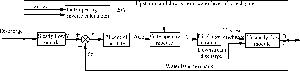
Figure 2. Canal automation control system

multireach serial canal system, under the condition of certain flow discharge, each canal reach should have its minimum restrained water level Zmin and maximal restrained water level Z . The target water level YT max varies with the variation of demanding discharge at canalside turnouts and canal downstream end in the control process and it is not a constant value. The controlled volume method of operation proposed in the paper adopts the real-time midpoint-weighted value of water level of canal reach upstream and downstream end, as the real-time target water level of the water level feedback control. Correspondingly with this, the initial target water level subtracts and adds on an allowable water level amplitude of variation, namely it is the minimum restrained water level Zmin and maximal restrained water level Z of the controlled volume max operation. The allowable water level amplitude of variation can be properly selected according to the canalside turnout constraint and the canal freeboard constraint. From analysis we can see that, different canal pool volume corresponds to the different midpoint-weighted water level of this canal pool. Therefore, the variation range of canal pool storage volume of controlled volume operation is situated through the setup of different limiting water level of canal pool.

When the most downstream end of canal has discharge demand variation, then the controlled volume operation regulation needs be carried through to the whole canal, which is the controlled volume operation of whole canal pools.

A.    Regulation of Discharge Difference

Supposes the initial total demand of discharge for the entire canal system is:

n

Q con = Q do + 2 Q o ( i )                (5)

i = 1

The total demand of discharge in other time for canal system is:

n

^Qsum = ^Qdown ⁺ E ^Qout ( i )                ⁽⁶⁾

i = 1

Then the variation of the total demand of discharge, namely the discharge difference is:

Qlack   Qsum

Q con

Where Q_do is the water taking discharge at the canal downstream end under initial state, Q o ( i ) is the water diversion discharge at each canalside turnout under initial state. Q_down and Q_out ( i ) are the water taking discharge at the canal downstream end and the water diversion discharge at each canalside turnout in other time, respectively. Actually, each canal pool may have more than one turnout, in order to be abbreviated expression, Q_out ( i ) represents the total water taking discharge in canal pool i ( i = 1,2..., n - 1, n ).

Then the discharge difference between the inflow and outflow in each canal pool is:

_i_             , V^j( i )

q lack ⁽ i ) = R t ^X Q lack ^X ~--------

2 v^j ( i )

i = 1

Where q_lack^j ( i ) is the assigned discharge difference of canal pool i in the time ^j , Q_lock^j = Q J - Q con , and Q_lack is the discharge difference between the real-time total demand of discharge and its initial value. V^j ' ( i ) is the storage volume of canal pool i in the time j . R_t is the weighting coefficient of discharge difference in the first round storage volume regulation, R_t e (0, 1], and it determines directly the strong or weak degree of the volume regulation, and enables the rulers to control the volume regulation speed according to requirements.

From the downstream end canal pool n to the upstream canal pool i ( i = n - 1 , n - 2 , "• 2,1), the upstream and downstream gate discharge of each canal pool are in turn:

Qu ( n ) = Qout ( n ) + Qdown - qiack (n)

Qd (n ) = Qdown(10)

Qu (i ) = Qout (i)+Qu (i+1)- qiack (i)

Qd (i ) = Qu (i +1)

The upstream and downstream gate discharge of each canal pool acquired through the controlled volume algorithm is namely the input variable of discharge feed forward in the controller of canal system.

B.    Real-time Target Water Level Calcalation

The water volume is a variable under the controlled volume method of operation, and the flow state in canal pool varies with the variation of discharge demand at the canal downstream end and canalside turnouts. According to the discharge difference of each canal pool, within the sampling period j , the variation of water volume for canal pool i is:

DV^J ( i ) = q lacck ( i ) ^x DT                 (13)

Then the new water volume of canal pool i is:

VC ( i ) = VC ^{- 1} ( i ) + DV^j ( i )             (14)

Where VC ^{- 1} ( i ) is the water volume of the last calculation period of canal pool, if the last calculation period is the initial time, then VC ^{- 1} ( i ) = V 0 ( i ) , DT is the calculation period.

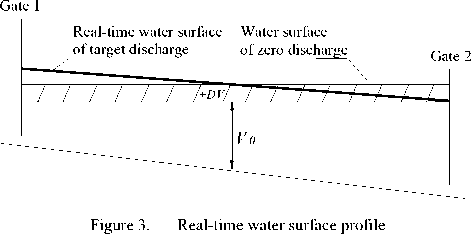
When there is new water volume of each canal pool, the water surface profile position of zero flow rate can be determined under this water volume. And then according to the target discharge state of corresponding time determined by discharge difference dispatching, then the singular target water surface profile of this time is determined. In the process of computer control operation, the real-time midpoint-weighted water level can be ascertained according to following method: firstly, supposes a downstream end water level of a canan pool, then uses the steady flow calculation module to calculate the water surface profile, and then the canal pool volume correspondingly to this supposed water level can be acquired, and the comparison is made between this volume with the real-time target volume computed by (14). If both are equal, then the supposed downstream water level is correct, otherwise, supposes the downstream end water level and calculates corresponding canal pool volume over again until the result is equal to the real-time target volume of this time. We can use the dichotomy method to carry on above iterative calculation.

When there is new real-time target water level and the real-time water level information derived from the unsteady flow calculation, the real-time water level difference can be acquired, and then it is regarded as the input variable of feedback controller to perform water level feedback control.

C.    Determination of the Target Water Level and Restricted Water Level

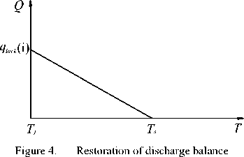
Both the target water level and target water volume of each canal pool under controlled volume operation can be regarded as the known values. Supposes the target water level of each canal pool is YT_tar ( i ) when canal system stabilizes, and the target water volume of each canal poo is V_tar ( i ). The restricted water levels of each canal pool are Z _min ( i ) and (or) Z _max ( i ) when the flow equilibrium regulation begins. Fig. 4 shows the linear reversion process of discharge difference, in which T_j is the time to begin the second round regulation, and the discharge difference between the inflow and outflow in each canal pool at this time is q_lack ( i ) , T s is the time to achieve equilibrium between the inflow and outflow. The time needed for linear subduction of discharge difference can be properly selected according to the stable requirement of system control. Usually the larger the discharge difference q_lack ( i ) is, the higher requirement of system stability is in the waterpower transient process of canal system, and the longer linear recovery time of discharge difference is needed.

Under the flow equilibrium regulation stage, the variation of water volume in each canal pool is:

A V ( i ) = 2 x q_lack ( i ) x ( T s - T)           (15)

Therefore, at the time when the flow equilibrium regulation begins, the water volume of each canal pool is:

V ( i ) = V- ( i ) -A V ( i )                 (16)

Author's study indicates the difference of the time to begin the flow equilibrium regulation for each canal pool is correspondingly small, and the discharge difference assigned to each canal pool is correspondingly smaller than the upstream gate discharge of this canal pool, so the upstream and downstream gate discharge of each canal pool from downstream end to upstream of canal system can be expressed approximately by (9)-(12) in turn when the flow equilibrium regulation begins.

Supposes when the flow equilibrium regulation begins, the discharge variation at each canalside turnout and canal downstream end has been stable, obviously, the discharge at upstream and downstream boundaries of each canal pool and each canalside turnout is known in this time. Because the beginning time of the flow equilibrium regulation for each canal pool may not be same, so there is certain difference between the actual rate flow and its calculation value at the upstream and downstream boundaries when the flow equilibrium regulation begins for each canal pool, but simulation indicates such difference is correspondingly small, and its influence on the target water level (or target water volume) calculation is very small, so the difference can be ignored

Before the simulation begins, according to the known water volume and discharge conditions of each canal pool when the flow equilibrium regulation begins, we can use the steady flow calculation module to calculate the singular water surface profile of each canal pool of this time, then the midpoint-weighted water level calculated from the upstream and downstream end water levels of this water surface profile is namely the restricted water level Z (i) or Z  (i) of each canal pool when min             max the flow equilibrium regulation begins.

D. Flow equilibrium regulation algorithm

When the real-time water volume of canal pool approaches the target volume VT ( i ) , the canal system needs to carry out the second round regulation to make the inflow and outflow of canal pool balanceable. Suppose the upstream gate flow rate of each canal pool is Q u ( i ) in the flow equilibrium regulation stage, the flow rate difference is q lack - t ( i ) when the flow equilibrium regulation begins, and the simulation period is DT . Then the calculation period times needed for accomplishing the flow equilibrium regulation of each canal pool is:

K n ( i ) =

T s

T j

DT

Where K_n ( i ) is the calculation period times needed to accomplish the flow equilibrium regulation of each canal pool; the meanings of other symbols are the same as the former.

Supposes the real-time calculation period number of each pool is K^j ( i ) at the flow equilibrium regulation stage, and the real-time recovery quantity of the flow rate difference of each pool is Q _sup ( i ) , then K^j ( i ) = 0 and Q _sup ( i ) = 0 in canal pools without flow equilibrium regulation, and 1 <  K^j ( i ) <  K n ( i ) in canal pools without flow equilibrium regulation.

If the canal pool has performed the flow equilibrium regulation, then its real-time recovery quantity of the flow rate difference is:

If 1 <  K^j ( i ) < K n ( i ) ,

^then Q sup ( i ) =

^K4 i ) K n ( i )

^X q lack - 1

( i )

If K ( i ) > K n ( i ) ,

^then Q sup ( i ) = q lack - 1 ( i )                                ⁽¹⁹⁾

At the flow equilibrium regulation stage, from the downstream end canal pool n to the upstream canal pool i ( i = n - 1 , n - 2 ,...2,1), the upstream and downstream gate discharge of each canal pool is in turn (all variables have abbreviated the time coordinates for simplification ):

Qu (n) = Qout (n)+Qdown - qM-1 (n)+Qsup (n)

Qd (n ) = Qdown(21)

n

Qu ( i ) = Z Qout ( k ) + Qdown n      k=i       n(22)

-E qlack-1 ( k ) + E Qsup ( k ) k=ik

Qd (i) = Qu (i +1)

The above gate discharge is namely the input variables of discharge feed forward in the controller of canal system at the flow equilibrium regulation stage.

E. Computational Example

• 1)    Basic Canal Conditions and Canal Reach Parameters

  The emergency water supply canal of the middle route of China south-to-north water transfers project is selected as the study canal. The starting point is the ancient canal check gate of Shijiazhuang city , the end point is the canal endpoint of Hebei province segment . The origin al stake number is 968 + 909, and the terminal stake number is 1196+167, the overall length of the simulation canal is 227.4 km. The entire canal system is divided into thirteen canal reaches by fourteen check gates; the design discharge is 170m³/s at the starting point, and 60m³/s at the end point. The canal system contains twelve canalside turnouts, sixteen inverted siphons , and three aqueducts, some under drains, culvert, bridges, transition sections and structures. The parameters of each canal pool see Table II.

In the study of this section, the upstream six canal reaches of the simulation canal is selected as the simulated object for simple ness (from canal pool 1 to canal pool 6 in Table I ). Then the end stake number of the simulated object is 1070 + 382, the overall length is 101.473km, the simulated object contains five canalside turnouts, six inverted siphons , one aqueduct, two under drains, one culvert and some transition sections and drainage structur es.

Because there are variation conditions of cross section forms and so on within the canal reaches, so each canal reach needs to be divided into some sub-reaches again. The division of interior sub-reaches and the calculation parameters see [11] for details. The canal roughness coefficient n = 0.015 .

• 2)    Parameters of the Inverted Siphons, Gates and Turnouts

The calculation methods and calculation coefficients of

head loss of inverted siphons in canal system see [12]. Because lacks some relevant parameters of gates in initial data, the useful width of each gate is supposed to be 20m referring to the connected structure width. The parameters of each turnout are shown in Table I .

TABLE I.      Parameters table of canalside turnouts

Turnout No.	Stake number	Position	Design discharge (m3/s)
1	982+418	pool 2	5
2	1006+048	pool 3	2
3	1029+321	pool 4	2
4	1034+575	pool 4	20
5	1059+925	pool 6	2
6	1068+925	pool 6	3
7	1102+941	pool 8	12
8	1116+185	pool 9	0.5
9	1120+325	pool 9	60
10	1154+975	pool 11	2
11	1179+272	pool 13	3
12	1194+291	pool 13	11

• 3)    Simulation Operating Condition and Results Analysis

The discharge at the canal downstream end decreases linearly from 80m3/s to 40m3/s in 1–3 hours, and the discharge at canalside turnouts decreases linearly from 100% design values to 40% design values in 1–3 hours.

Supposes the water depth at the most upstream end is 7.0m and maintains invariable. The initial condition of simulation is the steady flow state when the discharge at the canal downstream end and turnouts has not changed under the constant downstream depth operation.

The value of R_t is 0.7, the target water level YT_tar ( i ) is designed 0.3m above the initial midpoint-weighted water level. Then according to the accurate control method of water volume of the controlled volume operation, the restricted water level Z _max ( i ) of beginning the flow equilibrium regulation can be acquired, see Table Ш. If any canal pool has arrived at its restricted water level, then the linear recovery regulation of discharge difference is conducted for 2h for this canal pool to achieve the flow rate equilibrium between outflow and inflow. If all canal pools have achieved the flow rate equilibrium, then the water volume regulation of entire canal system is completed.

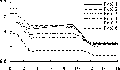
After the entire simulation process of the controlled volume operation is completed, the related characteristic parameters of volume variation of each canal pool are shown in Table Ш. The response processes of check gates see Fig. 5, the variation processes of gate discharge see Fig. 6, and the water level variation processes of part canal pools see Figs. 7–9. The control performance indicators [13] of canal operation see Table ^.

TABLE II.     Characteristic table of canal parameters

Canal pool No.	Number of inner sub-reaches	Length (m)	Design water depth (m)	Design discharge (m3/s)	Bottom altitude (m)
					Upstream end	Downstream end
1	5	9759	6.00	170	70.253	70.141
2	4	22053	5.00	170	69.991	69.032
3	4	15177	5.00	165	68.882	67.728
4	6	19553	5.00	155	67.578	66.475
5	3	9234	5.00	135	66.325	66.139
6	5	25697	4.50	135	65.989	64.935
7	3	13198	4.50	135	64.812	64.295
8	7	27098	4.50	135	64.145	61.486
9	4	9717	4.50	125	61.336	60.771
10	2	14924	4.50	100	60.621	59.920
11	5	20829	4.30	60	59.770	58.695
12	4	14705	4.30	60	58.545	57.849
13	8	25314	4.30	60	57.699	56.500

TABLE III.     The characteristic parameters of volume variation of each canal pool

Canal pool No.	Initial volume (106)	Steady volume (106)	Volume variation (106)	Z max (i)- YT (i) (m)	YT tar (i)- YT (i) (m)	q lack (m3/s)
1	1.23	1.34	0.10	0.264	0.298	-3.63
2	3.48	3.79	0.31	0.265	0.3	-10.25
3	2.16	2.35	0.19	0.265	0.302	-6.36
4	2.98	3.25	0.27	0.263	0.3	-8.79

5	1.19	1.30	0.11	0.267	0.298	-3.50
6	3.45	3.81	0.35	0.268	0.299	-10.18

(Note: YT (i) is the initial midpoint-weighted water level of each canal pool)

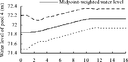
Figure 8. Water level variation processes of canal pool 4

Time (h)

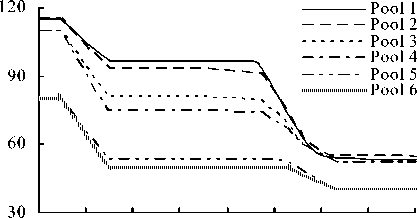
Figure 5. Upstream gate opening processes of each canal pool

Time (h)

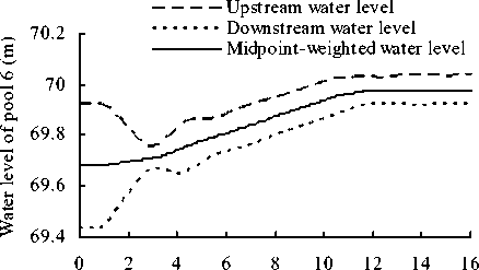
Figure 9. Water level variation processes of canal pool 6

0  2  4  6  8  10121416

Time (h)

TABLE IV.    Control performance indicators

Canal pool No.	MAE (%)	IAQ (m3/s)	IAW (m)	ISE (10-7m)
1	0.059	0.015	0.257	4.63
2	0.128	0.191	0.052	7.81
3	0.069	0.105	0.104	3.40
4	0.117	0.088	0.110	3.69
5	0.069	0.128	0.101	5.69
6	0.296	0.314	0.087	30.96

Figure 6. Upstream gate discharge processes of each canal pool

Time (h)

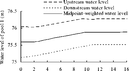
Figure 7. Water level variation processes of canal pool 1

Upstream water level

Downstream water level

Time (h)

The simulation results indicate:

• 1)    When the discharge demand at the canal downstream end and canalside turnouts decreases, in the first round regulation of check gates, uses the disequilibrium between outflow and inflow of canal pool to supply storage volume, and the water level of each canal pool ascends. The second round regulation of check gates makes the outflow and inflow of canal pool to be balanceable, and the water level tends to be stable.

• 2)    The water level indicators MAE and ISE of canal operation are relatively ideal, which indicates the system has good control effect over the water level. The values of subordinate performance indicators IAQ and IAW are very small, which indicates the processes of gate discharge and gate opening are also ideal in the process of system operation, and the gates have nearly not alternate motion.

• 3)    From the variation processes of gate opening we can see, the gate opening of the head of canal still has relatively obvious variation in the stable flow delivery stage when the absolute discharge difference has reached its maximum value (approximately in 3–9h). This is because the upstream water level of the head gate maintains constant, but the downstream water level of the head gate rises gradually along with the increase of water volume, therefore, the gate opening needs to increase gradually to maintain stable gate discharge.

• 4)    The canal system of the controlled volume method of operation proposed in the paper has very high

flexibility of operation and control. Through multi-rounds regulation, the water volume is rationally distributed according to proportion in time domain, it has guaranteed each canal pool to be effectively controlled regardless of the length of canal pool or participation of canalside turnouts. The midpoint-weighted water levels of all canal pools vary smoothly, the amplitude of water level fluctuation of upstream and downstream ends is also small. Moreover, the controlled volume algorithm proposed in the paper can comparatively accurately control the water volume or target water level of each canal pool (the absolute error of the stable target water level of each canal pool is less than or equal to 0.002m), therefore, the adjustable water volume of each canal pool is fully used.

• IV. Algorithm design of the Controlled Volume

Operation Method of Continuous Canal Pools

When the downstream continuous canal pools of canal system have no discharge demand change, and only some turnouts between canal head and middle canal pool of system have discharge demand change, if we adopt the controlled volume operation of whole canal system, it certainly will cause some unnecessary regulation, and consequently increases disturbed canal pools.

Therefore, when the discharge demand at some most downstream canal pools is invariable, and only some canalside turnouts between canal head and certain middle pool have discharge variation, then the most downstream pool which has discharge variation can be treated as an interior boundary, and the controlled volume regulation is made to this pool as well as all its upstream pools, all downstream pools of this pool can keep their original operation state and be invariable. When the most downstream discharge variation pool is closer to canal head, the advantage of this regulation method is more conspicuous. Therefore, the operation algorithm proposed is based on the assumption that some most downstream pools have no discharge variation, and when all canal pools of system have discharge variation, this algorithm can also be used directly.

A.    Regulation of discharge difference

Suppose the most downstream canal pool in which the discharge demand changes is the pool l (Fig. 10).

The calculation method s of Q_con , Q_sum and Q_lack are the same as above paragraph.

The discharge difference between the inflow and outflow in each canal pool is:

If l <  i <  n        qj ( i ) = 0                (24)

Vji

If 1 <  i <  l    q^ ( i ) = R x Q^ x -;AL  (25)

Z j i) i = 1

Where the meanings of all symbols are the same as above paragraph .

From the downstream end pool n to the upstream pool i ( i = n -1 , n - 2 ,...2,1), the upstream and downstream gate discharge of each pool are in turn:

If l <  i <  n :

Qu (i) = ZQo (k) + Qdown(26)

k = i

Qd (i —1) = Qu (i)

Qd (n) = Qdown(28)

If 1 <  i <  l :

Qu (i ) = Z Qout (k) + k=i(29)

nl Z Q o ( k ) + ^Qdown  Z q ack ( k )

k=l+1

Qd (i -1) = Qu (i)

B.    Flow Equilibrium regulation algorithm

At the discharge equilibrium regulation stage, from the downstream end pool n to upstream pool i , the upstream and downstream gate discharge of each pool are:

If l <  i <  n :

Qu (i ) = ZZ Qo (k)+Qdown(31)

Qd (i -1) = Qu (i)

Qd (n ) = Qdown(33)

If 1 <  i <  l :

ln

Qu (i ) = Z Qout (k )+Z Qo (k)+Qdown -k=ik ll

Z qack -1 (k )+Z Qsup (k) k=ik

Q d ( i - 1 ) = Q u ( i )

Where the meanings of all symbols are the same as the former.

The upstream and downstream discharge of each pool derived from the controlled volume algorithm are namely the input variables of the discharge feed forward control.

The real-time target point water level calculation, and the determination of the target water level and restricted water level see above paragraph.

C.    Computational Example

The thirteen canal reaches in the emergency water supply canal of the middle route of China south-to-north water transfers project is selected as the simulation canal. The overall parameters of simulated canal see Tables I and II.

The discharge at the canal downstream end is 30m3/s, and keeps invariable, the discharge at the Zhong Guantou turnout (belonging to canal pool 4 ) increases linearly from 5m3/s to 20m3/s in 1–5 hours, and other turnouts have no water intake discharge.

In the process of canal operation, only canal pool 1, 2, 3 and 4 participate in storage volume regulation, other pools keep their original operating state invariable.

The target water level YTtar (i) of canal pools with storage volume regulation are designed 0.15m below their initial midpoint-weighted water levels. Then according to the accurate control method of water volume, the restricted water level Zmin (i) can be acquired. If any pool has arrived at its restricted water level, then the linear recovery regulation of discharge difference is conducted for 2h for this pool to balance the final pool inflow and outflow. If all pools have achieved the flow rate equilibrium, then the water volume regulation of entire canal system is completed. The value of Rt is 0.7.

After the entire simulation process is completed, the related characteristic parameters of volume variation are shown in Table V. The response processes of check gates under the controlled volume operation of continuous canal pools and the controlled volume operation of whole canal system are shown in Fig. 11 and Fig. 12, respectively. The variation processes of gate discharge see Fig. 13, and the water level variation processes of part pools see Figs. 14–15. The performance indicators [13] of canal operation see Table И .

G(1)                     G(2) 11

Canal pool 1

V

Reservoir

Q u(i )

Canalside turnout ^Qout(1)

G( l )

Canal pool l g Qd(1)   Qu(2)

Q out( l -1)

Q out( l )

G( l +1 )

XI Qd( l )   M+1)

^G(n)                _rG(n+1)

Canal pool n

Q d(n-1) Q u(n)

I I Q o(n-1)

V

Q o(n)

Figure 10. Sketch map of canal system under controlled volume operation of continuous canal pools

TABLE V.     The characteristic parameters of volume variation of each canal pool

Canal pool No.	Initial volume (106 m3)	Steady volume (106 m3)	Volume variation (106 m3)	Initial target point water level (m)	Steady target point water level (m)	Variation of target point water level (m)
1	1.209	1.159	-0.050	75.515	75.364	-0.151
2	3.295	3.149	-0.146	74.106	73.958	-0.148
3	2.090	2.000	-0.091	73.058	72.908	-0.150
4	2.853	2.726	-0.127	71.672	71.521	-0.151
5	1.170	1.170	0	70.827	70.827	0
6	3.263	3.263	0	69.488	69.488	0
7	1.767	1.767	0	68.811	68.811	0
8	3.240	3.240	0	66.821	66.821	0
9	1.358	1.358	0	65.306	65.306	0
10	0.909	0.909	0	64.474	64.474	0
11	1.389	1.389	0	63.262	63.262	0
12	1.001	1.001	0	62.301	62.301	0
13	1.594	1.594	0	60.841	60.841	0

TABLE VI.    Control performance indicators

Canal pool No.	Controlled volume operation of continuous canal pools				Controlled volume operation of whole canal pools
	MAE (%)	IAQ (m3/s)	IAW (m)	ISE (10-8m)	MAE (%)	IAQ (m3/s)	IAW (m)	ISE (10-8m)
1	0.023	0.008	0.056	9.90	0.009	0.006	0.016	1.53
2	0.019	0.015	0.020	1.25	0.012	0.012	0.008	1.70
3	0.024	0.044	0.036	6.45	0.010	0.019	0.015	1.18
4	0.013	0.018	0.024	0.93	0.008	0.015	0.011	0.90
5	0	0.001	0.004	0.	0.008	13.122	0.265	1.02
6	0	0.001	0	0	0.022	12.132	0.181	5.57
7	0	0.001	0	0	0.008	9.415	0.183	0.66
8	0	0.001	0	0	0.014	7.940	0.116	2.42
9	0	0.002	0	0	0.011	5.238	0.106	1.41
10	0	0.001	0	0	0.014	4.094	0.091	0.56
11	0	0.001	0	0	0.015	3.335	0.075	2.76

0.001

0.015

2.175

0.057

2.82

1.2

0.001

0.031

1.320

0.028

11.88

1.1

о 0.9

0.8

0.7

^ 0.6

Я я

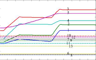
Figure 11. Upstream gate opening processes under the controlled volume operation of continuous canal pools

0   2   4   6   8 10 12 14 16 18 20 22 24

Time (h)

Figure 14. Water level variation processes of pool 4

0.5

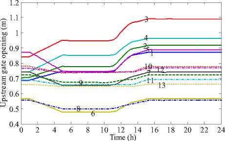
Figure 12. Upstream gate opening processes under the controlled volume operation of whole canal system

о 45 -45

71.1

70.9

70.8

70.7

5-13

250   2   4   6   8   10 12 14 16 18 20 22 24

Time (h)

Figure 13. Upstream gate discharge processes

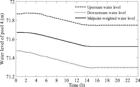
Upstream water level

Downstream water level

Midpoint-weighted water level

70.6 I----------------,----------------,----------------,----------------,----------------,----------------,----------------,----------------,----------------,----------------,----------------,----------------1

0   2   4   6   8   10  12  14  16  18  20  22  24

Time (h)

• Figure 15. Water level variation processes of pool 5

The simulation results indicate:

• 1)    When some downstream continuous canal pools have no demand change, the controlled volume algorithm proposed in the paper can realize controlled volume operation of continuous canal pools. The downstream continuous canal pools in which there is no discharge demand variation don’t participate in the water volume regulation, and keep their original operating state invariable, so the regulated check gates and disturbed canal pools are decreased, and the downstream continuous canal pools keep balanced water supply all the while. Especially, the closer of the most downstream discharge demand change canal pool is to the head of canal, namely the closer of l is to 1, the better control effect of this algorithm is.

• 2)    Because the most downstream turnout in which discharge demand changes belongs to canal pool 4, so canal pool 1, 2, 3 and 4 participated in controlled volume operation, and gate 1, 2, 3 and 4 are regulated according to the controlled volume algorithm. In order to guarantee constant discharge delivery, the gate 5 also should be adjusted according to its upstream and downstream water levels. The water level and discharge transition process es in regulated canal pools are relatively good, the same as the transition process es of regulated gates, so the control effect is relatively good. Because there is no discharge demand change from pool 5 to pool 13, they keep initial operating states invariable, so the number of disturbed canal pools and regulated gates is decreased.

• 3)    All performance indicators of regulated canal pools are slightly larger than the controlled volume operation of whole canal system, it is because that the target point water level variation is relatively larger under the controlled volume operation of continuous canal pools, and all performance indicators of other pools under this operation method is equal to or close to zero. The indicators IAW and IAQ of canal pools 5 to 13 under the controlled volume operation of whole canal system have relatively larger increase than pools 1 to 4, the reason for this is that the gates have reciprocating movement in pools 5 to 13, and discharge has certain

overshoot. All in all, the control effect of the controlled volume operation of continuous canal pools is better.

• 4)    Under the same operating conditions, the canal response time of the controlled volume operation of continuous canal pools is shorter than the controlled volume operation of whole canal system, it’s because the total discharge difference is distributed among lesser canal pools under the controlled volume operation of continuous canal pools, so the distributive discharge difference of each pool is relatively larger, and the time needed to accomplish the target storage volume regulation is shorter.

• V. CONCLUSION

The controlled volume method of operation is a more flexible canal operation method. This method of operation can fully use the adjustable water volume of canal; the canal water volume can be increased or decreased to buffer the rapid flow change to enhance the stability of canal operation. An operating simulation mode based on storage volume control method for multireach canal system in series under gate regulating is established in the paper. The algorithm of the controlled volume operation of whole canal pools was proposed, and the simulation to practical project indicates this method of operation can rapidly respond to discharge change of the canal downstream end and canalside turnouts, and can comparatively accurately control the water volume change. The variation of gate opening and water levels is comparatively smooth in the process of system operation, the control performance indicators of canal operation are very good; Furthermore, in allusion to some typical operating conditions, the algorithm of the controlled volume operation of continuous canal pools is proposed, the simulation to practical project indicates the new algorithm can relatively obviously reduce the number of regulated gates and disturbed canal pools, the control effect of canal system can be obviously improved. The controlled volume method of operation is especially suitable for long distance water transfer project, which lacks on-line regulation reservoirs but has larger canal pool storage. However, the controlled volume method of operation proposed in the paper has acquired good control effects only in non-ice period operation conditions. Under the dispatching operation of the ice period water delivery , the controlled volume method of operation needs to be made further study.

Acknowledgment