Research on SVG DC-Side Voltage Control Based-on PSO Algorithm

Published Online October 2016 in MECS

In recent years, the wide use of power electronic devices makes the semiconductor switching equipments increasingly diverse, these devices consume reactive power and bring additional burden for the power grid and adverse effects on the power quality. Therefore, it is important and urgent to control the reactive power in power grid in order to ensure the power transmission quality and ensure the power system to be effective, stable and normal operation.

SVG is a reactive power compensation device which composed of inverter, by controlling the on-off of the inverter switching device, continuous injection or absorption of reactive power to the power grid, not only can compensate reactive power, but also can compensate the harmonic[1-3].

At present, the efficiency of SVG in controlling reactive power, improving the power transmission quality and guarantying the power system stability and other aspects has been recognized. Because of its rapid development, it becomes one of the most important reactive power compensation devices, and is the focus of the research on the direction of reactive power compensation and harmonic control.

The main research contents of this paper mainly includes: (1) The operation flow of PSO algorithm is given, and the PSO algorithm and GA algorithm are applied to the optimization comparison of standard function extreme value[4-6]. (2) The inertia weight decreasing strategy of PSO is studied. (3) considering that the stability control of the DC side voltage is very important to guarantee the effect of SVG compensation, and considering the disadvantages of the traditional PI control with fixed parameters and the poor adaptability, the paper introduces the PSO algorithm with global search performance into the PI parameters optimization[7-9], online PSO-PI control and off-line PSO-PI control are obtained. (4) The paper takes the voltage loop of SVG as the controlled object, and the simulation verification is done for PSO-PI control.

• II.    Principle of SVG

According to the different choices of DC energy storage device, the SVG circuit can be divided into the voltage type bridge circuit and the current type bridge circuit, in fact, so far the used SVG mostly adopts the voltage type circuit, because the voltage type circuit has a high running efficiency. Therefore, SVG often refers to the voltage type circuit as the inverter circuit of dynamic compensation devices. The basic circuit structure is shown in Fig. 1.

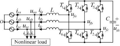
Fig.1. Basic circuit structure of SVG

The principle of SVG is that the AC side of inverter circuit can output the voltage u u u of preset fa ,fb ,fc amplitude and frequency through the on-off control of T~ T six semiconductor switching devices shown in Figure 1. Under the action of the connecting reactance, compensating current i ,i ,i are converted, and offset reactive current in power grid, achieve the purpose of reactive power compensation.

In practice, the IGBT full control switch is chosen as the semiconductor switching devices. Therefore, the SVG can be equivalent to the controllable amplitude and phase voltage source connected with the power grid through the connection reactance.

• III.    PSO Algorithm Research

  In 1995, Eberhart and Kennedy used the bird population behavior model of biologist Hepper to propose a particle swarm optimization (PSO) algorithm. Each individual in the group follows a very simple three rules of conduct:

• (1)    Away from the nearest individual, to avoid a collision.

• (2)    Flight to the target.

• (3)    Flight to the center of the group.

Different from the model proposed by Hepper, Kennedy thought birds initially didn’t know the target position, each individual follows a certain rule to evaluate their current position, and "local optimum" is used as the best position that it had flown, "globally optimal" is used as the best location that the entire population had flown, birds use the two optimal variables to guide their flight, share information with each other until the final flight target position.

Assuming there is a group of M particles, each particle is in a D dimensional search space, the speed of i particle can be expressed as vector v. = ( v._p v. ₂, • •• , v_iD ) , i = 1,2, ••• M , position is expressed as vector x. = ( x._px. , •••.,x._D ) . Then according to the pre-set fitness function, the merits of particles are evaluated for their current position, the position and speed of the particles are updated according to the fitness value, updated basis is two extreme values[10,11]: individual extremum and global extremum. The individual extremum is the best position of i particle to be found at present, denoted as pBest = ( p._p p ₂, • •• , p ^) . The global extremum is the best position to be found for all the particles in the group, denoted as gBest = ( p , p ₂, ••• , p _D), ( gBest is the optimal value of pBest ). For the k iteration, the update rule of particle speed and position in PSO is shown in the formula (1):

/ti¹ = ^k ⁺ c 1 r 1 ( Pd — x kd ) ⁺ c 2 r 2 ( !> .: — x kd )      (1)

* _X ^{k +1} = _X^k +v ^{k +1}

I x id     x id ^{+ v}id

In the formula (1), d = 1,2,•••,D , d represents the current search space dimension, i = 1,2, •••, M , i represents the particle, k represents the evolution algebra. xk : the d dimensional component of the position vector of particle i by k iterations. vk : the d dimensional component of the speed vector of particle i by k iterations. p : the d dimensional component of global extremum gBest . p : the d dimensional component of particle i individual extremum pBest . c , c : acceleration factor, c is used to adjust the particles speed flying to the individual extremum. c is used to adjust the particles speed flying to the global extremum. ro: inertia weight, adjust its size and can change the strength of the particle swarm search ability[12], r , r are the random number between [0,1].

• A.    PSO operation flow

The operation flow of PSO algorithm can be summarized as:

• 1.    Encoding for the solution space of problem

• 2.    Determining the objective function of optimization problem

• 3.    Initialization of the parameters in the algorithm

Common encoding way includes binary encoding and real encoding. Real encoding is more commonly used way of PSO algorithm encoding, and it directly searches the solution space.

The objective function is to reflect the characteristics of the problem to be optimized, that is, the fitness value of the particles. The fitness value of particles in the current position determines the update degree of the particle's position and speed.

• (1)    Determining the particle position and speed range, and initializing population size,

• (2)    Initializing the position information of each particle,

• (3)    Initializing the speed information of each particle,

• (4)    Initializing inertia factor, learning factor, iteration number and other parameters.

• 4.    Designing particle flying model

• 5.    Determining the termination condition of algorithm

• 6.    Code implementation

In the PSO algorithm, the flying speed of particles directly affects the ability of the particles to search for the optimal solution, too fast flying speed makes the particles fly over the global extreme point, and too slow flying speed may make particles falling into the local extreme point. The design of flying model directly reflects the ability of the particles to use their own memory and share the social information.

The termination condition of PSO algorithm is usually that the maximum number of iterations is satisfied or the fitness of the particles reaches a certain extreme value, also multiple termination conditions can be set according to different problems.

According to the above steps, the PSO algorithm is programmed, and need to change one or a few parameters of the algorithm in the process of debugging in order to search for the optimal solution.

Integrated the above steps, the PSO algorithm flow can be summarized as:

Step 1 : initialization of the algorithm parameters, initializing the population size, the number of iterations, the inertia weight, the learning factor, the particle position information and speed information et al.

Step 2 : according to the predetermined fitness function, the current fitness values of all particles are calculated.

Step 3 : compare the particle current position and individual extremum pBest , if the current position is better, the current position is used as the particle individual extremum pBest . Compare the current particle individual extremum pBest and group global extremum gBest , if the current position of the particle is better, the individual extreme pBest is used as the global extremum.

Step 4 : judging whether the termination of the algorithm is satisfied, if satisfied, the algorithm ends, if not satisfied, enter Step5.

Step 5 : each particle's position and speed are updated according to formula (1), continue to enter Step2.

• B.    Analysis of standard function simulation

• 1.    Simulation model

In order to show the superiority of the PSO algorithm, the PSO algorithm and GA algorithm are simulated in the same condition, and the solving efficiency of the two algorithms is compared.

Seeking the maximum value of Rosenbrock function in a certain range:

f ( x 1 , x 2 ) = 100 ( ^x1 ^- x 2 ) 2 + ( 1 ^- x 1 ) 2           (2)

• - 2.048 <  x <  2.048 ( i = 1,2 )

• 2.    Simulation parameter setting

  The sampling time of simulation t_s = 0.001 ₅ , the individual fitness is the value of Rosenbrock function, the reciprocal of the individual fitness is the objective function. The population size of GA algorithm Size = 500, termination of evolutionary algebra G = 200 , crossover probability p = 0.90    , mutation probability

• 3.    Simulation results

In the range of - 2.048 <  x , <  2.048 ( i = 1,2 ) , the function has two local extreme points, that is f ( 2.048, - 2.048 ) = 3897.7342    and     f ( - 2.048, - 2.048 ) = 3905.9262

respectively, and the latter is the global maximum.

P = 0.10 - [ 1:1: Size ] x 0.01/ Size , adaptive mutation probability, the smaller the adaptation degree, the greater the mutation probability, decimal encoding. PSO algorithm also uses the real encoding, group size, termination of the evolution algebra are same as GA algorithm, the particle speed range is [-0.1, 0.1].

Figure 2 shows the objective function values changes with the number of iterations for the GA algorithm and the PSO algorithm with linear decreasing strategy of inertia weight, it can be seen that the PSO algorithm has a faster convergence speed.

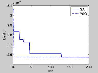
Fig.2. Optimization comparison between GA and PSO

According to the above simulation parameters, GA algorithm and PSO algorithm randomly run five times, the five results of GA are 3882.2210, 3860.4745, 3891.7978, 3878.3616, 3882.9877 respectively. While the five results of PSO are 3905.9262. It can be seen that the PSO algorithm has higher search accuracy and faster convergence speed, and has good stability.

In order to make the algorithm obtain the strong global search ability at the early, and the fast local convergence speed at the late, according to the formula (3) the inertia weight is reduced linearly. Among them, a Min , a Max are the minimum and the maximum inertia weight, iter is the number of the current iteration, iterMax is the total number of iterations.

a Max - a Min ro = a Max - iter x------------ ⁽³⁾

iterMax

In order to find a better balance between the global search ability and local search ability, two nonlinear inertia weight decreasing strategies are introduced into the paper, namely the concave function decreasing strategy and the convex function decreasing strategy, respectively, as shown in the formula (4) and formula (5):

a = ( a Max - a Min ) ( iter / iterMax ) ² +

(aMin - aMax) (2 iter / iterMax) + aMax a = -(aMax - aMin)(iter / iterMax )2 + aMax

In order to fully compare the influence on the global search ability and local search ability of PSO algorithm with three kinds of inertia weight decreasing strategies. Selecting, the group of particle swarm is 30, the number of iterations is 1000, the minimum value of the ten dimensional Rosenbrock function of formula (6) is searched, and the objective function is the function value.

f ( x 1, x 2 , ••• Х ц ) = ^ [ 100 ( x ² - x _w) 2 + ( 1 - x j² I

'                                 i =1 ^L

- 100 < x _y<  100 ( j = 1,2, ••• ,11 )

By using the convex function decreasing inertia weight and linear decreasing inertia weight and concave function decreasing inertia weight PSO algorithm, the minimum value of ten dimensional Rosenbrock function is searched respectively, and 50 times are done respectively. Three kinds of inertia weight decreasing strategies are used to obtain the minimum value of the function, the average value of 50 times is: 0.155331854735086, 0.123303231330160, 0.099328198916885. The fitness curve of PSO algorithm is shown in Figure 3 under three strategies. It can be seen that the PSO algorithm by using the concave function decreasing inertia weight has been accelerated, the inertia weight is reduced fast in the initial stage of the algorithm, and the convergence speed of the algorithm is accelerated, the optimization accuracy is the highest.

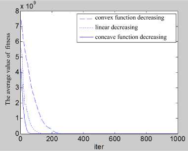
Fig.3. Comparison with three kinds of inertia weight decreasing optimization

• IV. PID Parameter Tuning based on PSO

The PSO algorithm is used for PID parameter tuning, according to the PSO algorithm tuning principle and the different ways of implementation, the tuning methods can be divided into off-line PSO-PID and on-line PSO-PID[13-18]. Figure 4 is the PSO-PID control system structure diagram.

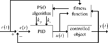
Fig.4. Control system structure of PSO-PID

• A.    Off-line PSO-PID algorithm

In off-line PSO-PID, PSO algorithm firstly needs off- line learning. The position and speed of the particles are updated within the scope of space according to the size of the fitness function, and constantly search for the optimal PID parameters, after the completion of the search, the global best position is substituted into the control system. In this paper, the time integral performance index of the error absolute value is selected as the fitness function, in order to prevent the overshoot and ensure the fast system response, the fitness function is shown in the formula (7).

J = ! > ( ^ e ( t )l ⁺ m 2 u ² ( t ) ) ^t ⁺ ® 3 t u (7)

In the formula (7), _e ( t ) represents the error, _u ( t ) represents the output of PID controller, t represents the rise time, ^ , m , ^ represent the weight of the performance index of each part.

The penalty function is introduced into the fitness function to prevent the overshoot. Once the overshoot is generated, the overshoot is used as the most important one of the fitness function. At this time, the fitness function is:

ife ( t ) < 0 j = j ( ^ 1 e ( t ) + m 2 u ² ( t ) + Ю 4 e ( t )^ t + ft ^ t u

In the formula (8), ^ □ m , in order to ensure that the adaptation value function is the largest proportion after the overshoot, that is, the current target is to suppress the overshoot.

After determining the fitness function, according to the PSO operation flow in MATLAB programming, the concave function decreasing strategy of the inertia weight is used, and the process of the off-line PSO-PID is as follows:

Step 1 : initialization of algorithm parameters. The population size, the iteration number, the inertia weight, the learning factor, the initial values of PID parameters, the update speed, the change range of the position & speed, and each weight value in formula (7) and (8) are initialized.

Step 2 : takes the each current particle PID parameters into the controlled object, gets the performance parameters of corresponding step response, calculates the fitness value of particles according to formula (7) and (8).

Step 3 : comparison between the current particle position and individual extreme pBest , if the current position is better, take the current position as the particle individual extreme pBest . Compare the current particle individual extremum pBest with the group global extremum gBest , if the current particle position is better, take the individual extreme pBest as the global extremum value.

Step 4 : judging whether the termination condition of the algorithm is satisfied. If satisfied, the algorithm ends. If not satisfied, enter Step5.

Step 5 : according to the formula (1), the position and speed of each particle is updated, continue to enter Step2.

In order to verify the effectiveness of the off-line PSO-PID algorithm, the two order transfer function of the formula (9) is used as an example, and the results are compared with the off-line GA-PID tuning value and offline PSO-PID tuning value.

Controlled object:

G ( s ) =

s ² + 50 s

Setting simulation parameters, the crossover probability and mutation probability of GA algorithm are 0.9, 0.033 respectively. In formula (7) and (8), ^ , ^ , ^ , ^ are 0.999, 0.001, 100, 2.0 respectively. The initial inertia weight of PSO algorithm is 0.95, the termination of inertia weight is 0.4, the concave function decreasing strategy is adopted, the acceleration factor q = _c = 2 . The range of proportional gain parameter of GA algorithm and PSO algorithm is [0,20], the integral gain parameter and the differential gain parameter are [0,1], the number of particles is 30, real encoding, 100 generations of iteration.

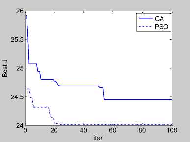
Fig.5. Adaptive value iteration curve of GA and PSO

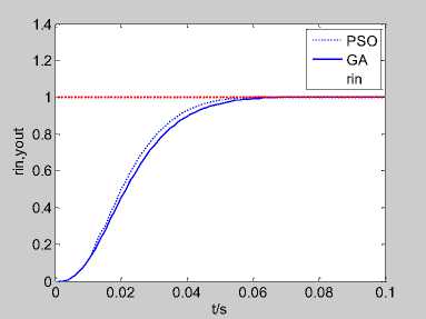
Fig.6. The step response of the system under the condition of off-line GA and off-line PSO

Figure 5 is the adaptive value iteration curve of GA and PSO, Figure 6 is the step response of controlled object by using two algorithms to find the optimal PID parameters. Can be seen that the PSO algorithm converges quickly fast, the optimal value can be found in 25 generations, but GA algorithm needs 54 generations around to find the optimal value. From the optimization accuracy, the final fitness value of PSO algorithm is 24.0122, the final fitness value of GA algorithm is 24.4478.

According to Figure 5 and Figure 6, GA algorithm and PSO algorithm can obtain better effect in the off-line tuning of PID parameters, the step response curve is basically no overshoot, and has fast rise time. Compared with GA algorithm, PSO algorithm has higher searching accuracy and better convergence speed, and the off-line PSO-PID has better tuning effect.

• B.    Online PSO-PID algorithm

The so-called online PSO-PID tuning method is to tune PID parameters at each sampling period. For example in a sampling time, select enough particles, calculate each individual's fitness, according to the degree of fitness the magnitude and direction of the particle position and speed updating value are determined, after a certain number of iterations, the optimal PID parameters are obtained at this sampling time. In the next sampling time, the optimal PID parameters are searched by using the same method.

Firstly, the particle fitness function is constructed, and the absolute value of the error and the absolute value of error change rate are used as the fitness function of i particle:

J ( i ) = a p x j errori ( i )| + P p x \de ( i )| ⁽¹⁰⁾

In the formula (10), _a^ , p are the weight, ermri ( i ) is the error of i particle, d_e ( i ) is the error change rate. The introduction of the penalty function is to prevent the overshoot:

if errori ( i ) < 0 J ( i ) = J ( i ) + 100 | errori ( i )| ⁽¹¹⁾

Online PSO-PID algorithm can be summarized as the following six steps:

Step 1 : Setting sampling time, initializing the size of the population, the number of iterations, the inertia weight, the learning factor and the initial value of the PID parameters and the update speed and the weight of the formula (10).

Step 2 : in the k sampling time, take the PID parameters of current each particle into the controlled object, calculate the error and error change rate, then calculate the fitness values according to formula (10) and (11).

Step 3: compare the particle current position and individual extremum pBest , if the current position is better, the current position is used as the particle individual extremum pBest . Compare the current particle individual extreme pBest and the global extremum gBest , if the current particle position is better, the individual extreme pBest is used as global extremum. The current best position is used as the PID parameters in the k sampling time.

Step 4 : judging whether to meet the algorithm termination conditions in this sampling time, if satisfied, jump into Step6. If not satisfied, enter Step5.

Step 5 : follow the formula (1) to update the particle position and speed, and then continue to enter Step2.

Step 6 : judge whether the final time of algorithm is satisfied or not, if satisfied, the algorithm ends. If not satisfied, k = k + 1, enter the next sampling time, enter Step2.

Also select formula (9) as the controlled object, the system input is the step signal, sampling time is 1ms, PD parameters are optimized on-line by PSO algorithm and GA algorithm. Proportional gain parameter range is [9.0, 12.0], differential gain parameter range is [0.2, 0.3], GA algorithm crossover probability p = 0.90 , mutation probability p = 0.20 - [ 1:1: Size ] x 0.01/ Size , the initial inertia weight of PSO algorithm is 0.95, the termination of the inertia weight is 0.4, concave function decreasing strategy, acceleration factor _c = c ₂ = 2 ■ The population size of two algorithms is 120, the generation of evolutionary algebra is 10, use formula (10) and (11) as the fitness function, and a p = 0.95, P p = 0.05 ■

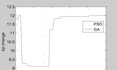
Figure 7 is the step response curve by using on-line PSO-PD and on-line GA-PD to optimize PD parameters, figure 8 respectively represents the varying curve of two algorithms under the proportional gain k and the differential gain k versus time. Can be seen from Figure 8, k and k have similar time varying trend under two kinds of algorithms.

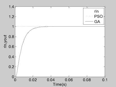
Fig.7. The system step response under the condition of online GA and online PSO

For the two cases of off-line PID tuning and on-line PID tuning, after a comprehensive comparison, the application of GA algorithm and PSO algorithm in PID parameters tuning can be concluded as follows:

• (1)    Compared with the off-line GA-PID, off-line PSO-PID has faster convergence speed and higher searching accuracy.

• (2)    The step response of the system is almost the same at on-line GA-PID and on-line PSO-PID tuning. Because the PSO algorithm has no selection, crossover and mutation operators in GA algorithm, it only needs to update the position and speed information according to the adaptive value, so the algorithm is simpler and faster.

• (3)    Compare figure 6 and figure 7, the step response of on-line tuning is better than that of off-line tuning.

8.5

0       0.02     0.04     0.06     0.08      0.1

Time(s)

(a) Proportional gain parameter variation

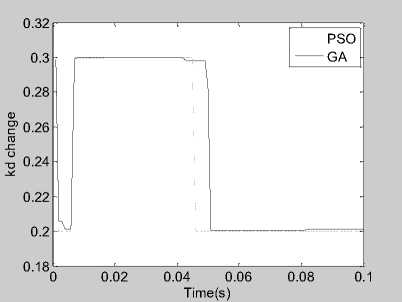
(b) Differential gain parameter variation

Fig.8. Parameters variation waveform of online GA and online PSO

• V.    Research on SVG DC-Side Voltage Control

In theory, SVG by using full control device, which is used to the reactive power compensation of the power grid, is not required to set up the energy storage element in the DC side. But in practice, considering the SVG converter circuit to absorb the fundamental current in addition, but also including harmonic current, which will cause the round return of part energy between the SVG and the power supply. Therefore, the existence of the DC energy storage elements can guarantee the stability of the converter circuit[19-23], actually the SVG has both reactive power compensation and low order harmonic compensation function.

• A.    Energy exchange between SVG DC side and AC side

The following is an analysis of the energy exchange between the DC side and the AC side of SVG in the reactive power and harmonic compensation[24-28].

For SVG system, the instantaneous active power and instantaneous reactive power of the power side are represented by p and q respectively, p and q are used to represent the instantaneous active power and instantaneous reactive power of SVG output, the instantaneous active power and instantaneous reactive power of the load side are represented by p and q . Considering that the load current contains a partial harmonic, p and q can be expressed as:

| P l = ^pL + Pl               (12)

1 q L = q L + q L

In the formula (12), p and q represent the DC component of active power and reactive power in the load, p and q represent the AC component of active power and reactive power in the load.

When only reactive power compensation with SVG:

p SVG = ⁰ q SVG = - q L

At this time:

P s = P l + P svg = P l + ^pL . 4 s = q L + q SVG = 0

There is no active energy exchange between the SVG DC side and the AC side, and the DC side voltage should be kept constant. In theory, the DC side does not need energy storage element at this time.

When the harmonic is only compensated:

P sVG = - ^pL q SVG = - q L

P svg = ^{- p}_L q SVG = - q L

At this time:

P s = P l + P svg = P l q s = ^qL + q SVG = ⁰

At this point, the voltage of the DC side will fluctuate and is similar to that of the harmonic only when it is compensated. In fact, whether it is the compensation of harmonic or reactive power, the system itself has a loss. The power loss of SVG mainly includes the loss of the inverter switching device and the magnetic hysteresis loss of the output inductor, copper loss, etc. In the case of the switching frequency, the power loss of SVG increases with the increase of the DC side voltage. The above analysis shows that the DC side voltage will change in the working process of SVG, in order to guarantee the stability of the SVG compensation performance and low power loss, the DC side voltage must be controlled [2931].

• B.    Derivation of voltage loop transfer function

For the control of DC side voltage, at present, it is used to add a voltage outer loop on the basic of the current tracking control inner loop. Figure 1 is the SVG basic circuit structure, with this figure as the object, the transfer function of SVG DC side voltage loop is derived.

In figure 1, usa, usb and usc represent the power grid three-phase voltage, i,i   and i   represent the grid side three-phase current, i,i and i represent the SVG output three-phase current, uu   and  u fa, fb               fc represent the three-phase voltage of the PWM inverter output, u represents the capacitor voltage of SVG DC side. The connecting inductor is L and the DC side capacitance is C .

Assuming the power grid is three phase equilibrium, the fundamental electric potential of three-phase power grid is:

At this time:

P s = P l + P svg = P l . q s = q L + q SVG = q L

At this point, SVG is needed to provide active energy, the average value of instantaneous active power is zero, but there is the AC component in p , DC side voltage will fluctuate with p .

When the reactive power and harmonic are compensated at the same time:

'u sa = ^Em c^Os( ® t )

< u_sb = E_m cos( a t - 120°)

_ u sc = E m cos( ® t + 120°)

Considering that the switching frequency is high, it is much higher than the grid frequency, only considering the low frequency component of the switching function s_k ( k = _a , b , c ) , the PWM harmonic components are ignored[20], then:

s_a « 0.5 m cos ( ro t - ^ ) + 0.5

< s_b ® 0.5 m cos ( ro t - 9 - 120° ) + 0.5 s_c « 0.5 m cos ( ro t - 9 + 120° ) + 0.5

In the formula (20), 0 represents the initial phase angle of the fundamental wave for the switching function, m represents the PWM modulation ratio ( _m <  1 ) .

Three phases grid side current is:

i sa ” I m cos (. m t )

‘ i sb ” I m cos ( ro t - 120° ) _ i se ~ I m cos (mt +¹²⁰ )

The other three phases DC current can be described as a switching function:

i = sJ™ + sJ, + sj„ dc     a sa     b sb     c sc

Taking formula (20) and (21) into formula (22), the DC side current of the inverter circuit and the grid side current simplified model are obtained as follow:

ide ~ 0.75 mI m ^cos 0

According to the formula (23), the SVG voltage loop structure diagram is shown in Figure 9. Without considering the load current i disturbance, the voltage loop transfer function can be expressed as follow:

0.75 m cos 0

”^Л s > = ( , . + T . ) 0, 2 + Cs

In the formula (24), у ( 1 ₊ ^ _s ) is the small inertial delay for the sampling of DC side voltage, W_ci ( s ) - 1 ( 1 ₊ T_cis ) is the current inner loop equivalent function, 0.75 m cos 0 is a time varying link that represents the relationship between the DC side current and the grid side current, and the controlled object is a time-varying system, in most references, 0.75 m cos 0 is reduced to 0.75 ( m <  1 ) , the controlled object is simplified as constant system.

W V ( s ) =

0.75

( t_v + T_d) Cs ² + Cs

In order to compare the performance of the traditional PI control system with the time varying system and the constant system, the time varying link K = 1 + 0.1sin 2 n t is added in the constant system of formula (25).

W Ov ( s ) =

0.75 K

T v + T ei .) Cs ² + Cs

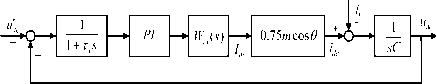
Fig.9. SVG voltage loop structure diagram

• C.    DC side voltage control based on PSO

  In the paper, for the constant system of formula (25) and the time varying system of formula (26), simulation is done respectively to verify the control effect of the traditional PI control system and time varying system. In practice, ( ^ ₊ T_c .) takes 0.08s, DC side capacitance C takes 0.0022 F .

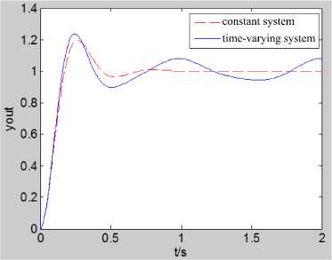
Fig.10. The step response of traditional PI control in constant system and time-varying system

Figure 10 is the unit step response of the traditional PI control for the constant system and time varying system, k p and k are derived from the classical Z-N method, k p = 0.0446, k. = 0.0021. The unit step response index of the constant system of formula (25) in traditional PI control is that overshoot =20.8%, the rise time =0.1133s, steady output y=1.005. The unit step response index of the time varying system of formula (26) in traditional PI control is that overshoot =22.5%, the rise time =0.1038s, steady output y =0.9507~1.0963. Obviously, traditional PI control for the constant system has better dynamic response characteristics, and the output basically has no steady-state error. However, when the system parameters are variable, the overshoot is obviously increased, and there is the output oscillation and steady-state error.

For the time varying system of formula (26), the PI parameters are optimized by using the off-line PSO and the on-line PSO algorithm respectively. The initial inertia weight of PSO algorithm is 0.95, the termination of the inertia weight is 0.4, the concave function decreasing strategy is used, acceleration factor . = e ₂ = 2 , the algorithm population size is 120, the evolutionary algebra is the 10 generations, speed range is set to [- 1,1], the range of k is [0,10], the range of k is [0,1]. Uses the formula (10) and (11) as the fitness function, and a _p = 0.95, p _p = 0.05.

Figure 11 is the unit step response of time-varying system by using three control methods, and the corresponding response index is shown in table 1. Compared with the traditional PI control, the overshoot of off-line PSO-PI control is reduced, the rise time is faster, but its essence is still the PI control, so system output has oscillation, although steady-state error problem has eased, but has not yet been resolved. While the unit step response of on-line PSO-PI control has a faster response time, almost no overshoot, no output oscillation, and steady error is almost zero, it has strong adaptability for time varying system.

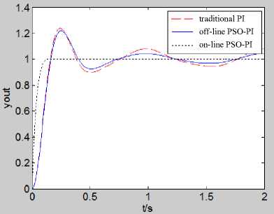
Fig.11. The step response of three control methods in time-varying system

Table 1. The step response performance index under three control modes

	k p	ki	σ /%	t r /s	y
traditional PI	0.0446	0.0021	22.5	0.1038	0.9507~1.0963
off-line PSO-PI	0.0421	0.0013	20.56	0.1094	0.9671~1.0354
on-line PSO-PI	variation	variation	0.2	0.0295	1.0003

• VI.    Conclusions

With the development of power electronic devices, the load form in the power grid is becoming more and more diversified, which leads to the severe low power factor. In the field of reactive power compensation, SVG with fast response speed, smooth adjustment of reactive power, reliable operating characteristics and high precision becomes the new research hotspot in the field of reactive power compensation, represents the development direction of reactive power compensation device.

Because the stability control of the DC side voltage is very important for the SVG compensation effect, considering the disadvantages of the traditional PID control with fixed parameters and the poor adaptability[32-36], the paper introduces the PSO algorithm with global search performance into the PI parameters optimization. The paper takes the SVG voltage loop as the controlled object, and the voltage loop transfer function is deduced. Combined with PSO algorithm, on-line PSO-PI control and off-line PSO-PI control are adopted, and decreasing strategy of inertia weight function is used. The simulation results show that PSO-PI control can satisfy the situation of time varying system, and has strong adaptability.

Acknowledgment

The authors wish to thank my graduate tutor Hongbin

Wu Professor and Benxian Xiao Professor and graduate student Qinglin Zhang and Peng Zhang.