Review and Comparison of Kernel Based Fuzzy Image Segmentation Techniques

Published Online June 2012 in MECS

Image segmentation plays an important role in image analysis and computer vision. The goal of image segmentation is partitioning of an image into a set of disjoint regions with uniform and homogeneous attributes such as intensity, color, tone etc. The image segmentation approaches can be divided into four categories: thresholding, clustering, edge detection, and region extraction. In image processing, two terms are usually seen very close to each other: clustering and segmentation. When we analyze the color information of the image, e.g. trying to separate regions or ranges of color components having same characteristics, the process is called color clustering and mapping the clusters onto the spatial domain by physically separated regions in the image is called segmentation. In images, the boundaries between objects are blurred and distorted due to the imaging acquisition process. Furthermore, object definitions are not always crisp and knowledge about the objects in a scene may be vague. Fuzzy set theory and Fuzzy logic are ideally suited to deal with such uncertainties. Fuzzy sets were introduced in 1265 by LoftiZadeh[1] with a view to reconcile mathematical modeling and human knowledge in the engineering sciences. Medical images generally have limited spatial resolution, poor contrast, noise, and non-uniform intensity variation. The Fuzzy C- means (FCM) [5], algorithm, proposed by Bezdek, is the most widely used algorithm in image segmentation because it has robust characteristics for ambiguity and it can retain much more information than hard segmentation methods. FCM has been successfully applied to feature analysis, clustering, and classifier designs in fields such as astronomy, geology, medical imaging, target recognition, and image segmentation. An image can be represented in various feature spaces and the FCM algorithm classifies the image by grouping similar data points in the feature space into clusters. In case the image is noisy or distorted then FCM technique wrongly classify noisy pixels because of its abnormal feature data which is the major limitation of FCM. Various approaches are proposed by researchers to compensate this drawback of FCM.

Tolias and Panas developed a rule based system that post-processed the membership function of any clustering result by imposing spatial continuity constraints and by using the inherent correlation of an eight-connected neighborhood to smooth the noise effect[6]. Acton and Mukherjee[7] incorporated multiscale information to enforce spatial constraints. Dave[1] proposed the idea of a noise cluster to deal with noisy data using the technique, known as Noise Clustering. He separated the noise into one cluster but this technique is not suitable for image segmentation, as we cannot separate pixels from the image. Another similar technique, PCM, proposed by Krishnapuran and Keller[2] interpreted clustering as a possibilistic partition. However, it caused clustering being stuck in one or two clusters. Ahmed et al.[10] modified the objective function of FCM by introducing a term that allowed the labeling of a pixel to be influenced by the labels in its immediate neighborhood. Zhang Yang, Fu-lai Chuang et al. (2002)[11] developed a robust clustering technique by deriving a novel objective function for FCM. Jiayin Kang et al.[12] proposed another technique which modified FCM objective function by incorporating the spatial neighborhood information into the standard FCM algorithm. Y. Yang et al.[13] proposed a novel penelized FCM (PFCM) for image segmentation where penalty term acts as a regulizer in the algorithm which is inspired by neighborhood maximization (NEM) algorithm[14] and is modified in order to satisfy the criterion of FCM algorithm. S. Shen, W. Sandham et al. [15] presented an algorithm called Improved FCM which changed the distance function used in FCM, i.e. the distance between pixel intensity and cluster intensities, and applied neural network optimization technique to adjust parameters in the modified distance function. Keh-Shih Chuang, Hong-Long Tzeng et al. [16] presented a FCM algorithm that incorporated spatial information into the membership function of clustering. The membership weighting of each cluster is altered after the cluster distribution in the neighborhood is considered. Rhee and Hwang [17] proposed Type 2 fuzzy clustering. Type 2 fuzzy set is the fuzziness in a fuzzy set. In this algorithm, the membership value of each pattern in the image is extended as type 2 fuzzy memberships by assigning membership grades (triangular membership function) to Type 1 fuzzy membership. The membership values for the Type 2 membership matrix are obtained as:

^ik = ^- (1)

Where a ik and u ik are the Type 2 and Type 1 fuzzy membership respectively. The cluster centers are updated according to the conventional FCM by taking into account the new Type 2 fuzzy membership.

While discussing the uncertainty, another uncertainty arised, which is the hesitation in defining the membership function of the pixels of an image. Since the membership degrees are imprecise and it varies on person’s choice, hence there is some kind of hesitation present which arised from the lack of precise knowledge in defining the membership function. This idea lead to another higher order fuzzy set called intuitionistic fuzzy set which was introduced by Atanassov’s[4] in 1213. It took into account the membership degree as well as non-membership degree. Few works on clustering is reported in the literature on intuitionistic fuzzy sets. Zhang and Chen (2002) suggested a clustering approach where an intuitionistic fuzzy similarity matrix is transformed to interval valued fuzzy matrix. From the similarity degrees between two intuitionistic fuzzy sets, intuitionistic fuzzy similarity matrix is created which is transformed to intuitionistic fuzzy equivalence matrix. Then, a clustering technique that uses intuitionistic fuzzy equivalence matrix is suggested based on the λ-cutting matrix of the intuitionistic fuzzy equivalence matrix. Recently, T. Chaira [2] proposed a novel intuitionistic fuzzy c-means algorithm using intuitionistic fuzzy set theory. This algorithm incorporated another uncertainty factor which is the hesitation degree that arised while defining the membership function.

This paper provides a comparative study of the original Fuzzy c- means clustering algorithm and its three kernalized variations like kernel based fuzzy c-means (KFCM),kernel based intuitionistic fuzzy c-means (KIFCM),kernel based Type-2 FCM (KT2FCM) which are the kernalized extension of their non kernalized counterparts FCM,IFCM and T2FCM respectively. The algorithms are kernalized by adopting a kernel induced metric in the data space to replace the original Euclidean norm metric. By replacing the inner product with an appropriate ‘kernel’ function, one can implicitly perform a non-linear mapping to a high dimensional feature space in which the data is more clearly separable.

The organization of the paper is as follows: Section II reviews Fuzzy C-Means (FCM), Kernelized Fuzzy C-Means (KFCM), Kernelized Type-2 FCM (KT2FCM) and KernelizedIntuitionistic Fuzzy C-means (KIFCM) in detail. Section III evaluates the performance of the algorithms presenting a comparison between them both qualitatively and quantitatively followed by conclusion in section IV.

• II.    Background Information

This section discusses the Fuzzy C-Means (FCM), Kernelized Fuzzy C-Means (KFCM), Kernelized Type-2 Fuzzy C-means(KT2FCM), and Kernelized Intuitionistic Fuzzy C means (KIFCM) algorithms in detail. In this paper, the data-set is denoted by ‘X’, where X={x 1 , x 2 , x 3 …x n } specifying an image with ‘n’ pixels in M-dimensional space to be partitioned into ‘c’ clusters. Centroids of clusters are denoted by v i and d ik is the distance between x k and v i .

• A. Kernel based approach

The present work proposes a way of increasing the accuracy of the intuitionistic fuzzy c-means by exploiting a kernel function in calculating the distance of data point from the cluster centers i.e. mapping the data points from the input space to a high dimensional space in which the distance is measured using a Radial basis kernel function.

The kernel function can be applied to any algorithm that solely depends on the dot product between two vectors. Wherever a dot product is used, it is replaced by a kernel function. When done, linear algorithms are transformed into non-linear algorithms. Those nonlinear algorithms are equivalent to their linear originals operating in the range space of a feature space φ. However, because kernels are used, the φ function does not need to be ever explicitly computed. This is highly desirable, as sometimes our higher-dimensional feature space could even be infinite-dimensional and thus infeasible to compute.

A kernel function is a generalization of the distance metric that measures the distance between two data points as the data points are mapped into a high dimensional space in which they are more clearly separable. By employing a mapping function Φ( X ), which defines a non-linear transformation: X →Φ( X ), the non-linearly separable data structure existing in the original data space can possibly be mapped into a linearly separable case in the higher dimensional feature space.

Given an unlabeled data set X={x1, x2, …., xn} in the p-dimensional space RP, let Φ be a non-linear mapping function from this input space to a high dimensional feature space H:

Φ: Rp →H, x→Φ(x)

The key notion in kernel based learning is that mapping function Φ need not be explicitly specified. The dot product in the high dimensional feature space can be calculated through the kernel function К ( Х[ , Xj ) in the input space R^P.

K(xi,xj)=Φ(хi). Φ(xj)

Consider the following example. For p=2 and the mapping function Φ,

Φ: R² → H =   ( %И ^, ^/2)→( X^ ^{, x}i2 ,√2 ХцХ₁₂ )

Then the dot product in the feature space H is calculated as

RBF function with a=1, b=2 reduces to Gaussian function.

Example 4: Hyper Tangent Kernel:

К ( ■^t ^, Xj )=

-

‖Xi~Xj‖ tanℎ(-‖    ‖ ),

where a >0

Φ(Xi).Φ(Xj )

= ( ^xii , ^xi2 ,√2 ХцХ₁₂ )․( X^i , Xj2 ,√2 ХцХ₎₂ )

= ((xh , xi2).(Xji, Xj2 )) 2

= ( ^i . Xj )2

= (Xi , Xj )

where K-function is the square of the dot product in the input space. We saw from this example that use of the kernel function makes it possible to calculate the value of dot product in the feature space H without explicitly calculating the mapping function Φ. Some examples of kernel function are:

Example 1: Polynomial Kernel:

К ( Xi , Xj )=( Xi . Xj + c ) d , where c≥0, й ∈ N

Example 2: Gaussian Kernel:

B. The Fuzzy C Means Algorithm (FCM)

Fuzzy c-means (FCM)[1] is a method of clustering which allows one piece of data to belong to two or more clusters. This method (developed by Dunn in 1273 and improved by Bezdek in 1211) is frequently used in pattern recognition. FCM is the most popular fuzzy clustering algorithm. It assumes that number of clusters ‘c’ is known in priori and minimizes the objective function (J FCM ) as:

c n

/fcm =∑∑uik ‖ Xk - Vi ‖2 ,1≤m<∞Jfcm i=l k=l c n

=∑∑ ^uik^ik i=l k=l

0≤Utk ≤ 1for all i , k ;(2a)

∑1=1 ^ik=1 for all k;(2b)

∑ k=lUik>0 ∀i(2c)

Where^ik =‖Xr -  ‖, and uik is the membership of pixel ‘xk’ in cluster ‘i’, which satisfies the following relationship:

∑1=1 ^ik=1; i=1,2,…․․n(3)

Here ‘m’ is a constant, known as the fuzzifier (or fuzziness index), which controls the fuzziness of the resulting partitionand can be any real number greater than 1 but generally we take it as 2 . Any norm ‖·‖expressing the similarity between any measured data and the centre can be used for calculating d ik . Minimization of J FCM is performed by a fixed point iteration scheme known as the alternating optimization technique. This algorithm works by assigning membership to each data point corresponding to each cluster centre on the basis of distance between the cluster centre and the data point. More the data is near to the cluster centre more is its membership towards the particular cluster centre. Clearly, summation of membership of each data point should be equal to one.The conditions for local extreme for (1) and (2) are derived using Lagrangian multipliers:

К(xt , XJ)=exp

(-‖xt"xi ‖

(- ^ ),

where a >0

Example 3: Radial basis Kernel:

к(xt , xj)=exp

∑|x^-x^|

(-        ), where a , a , b >0

Uik =                                       (4)

∑   ( ^‖ 4zjjk ‖

∑   (‖ Xj-Vk‖)

^ik =               ∀к,i(5)

∑ ^(%)

where1 ≤ i ≤ c ; 1≤ к ≤ n and

Vi =∑  ( $) ∀i(6)

∑k=i(uik)

The FCM algorithm iteratively optimizes J FCM (U,V) with the continuous update of U and V, until |U^(l+1) – U^(l)| <= ε, where ‘l’ is the number of iterations. FCM works fine for the images which are not corrupted with noise but if the image is noisy or distorted then it wrongly classifies noisy pixels because of its abnormal feature data which is pixel intensity in the case of images, and results in an incorrect membership and improper segmentation.

Algorithmic steps for Fuzzy c-means clustering

Let X = {x 1 , x 2 , x 3 ..., x n } be the set of data points and V = {v 1 , v 2 , v 3 ..., v c } be the set of centers.

• 1)    Randomly select ‘c’ cluster centers.

• 2)    Calculate the fuzzy membership 'µ ij ' using:eq(4)

• 3)    Compute the fuzzy centers 'v j ' using:eq(6)

• 4)    Repeat step 2) and 3) until the minimum 'J' value is achieved or ||U(k+1) - U(k)|| < ε.

where‘k’ is the iteration step.

‘ε.’ is the termination criterion between [0, 1].

• C.    Kernelized Fuzzy c-means (KFCM)

Fuzzy C-means (FCM) [3] clustering algorithm is the soft extension of the traditional hard C-means. It considers each cluster as a fuzzy set, while a membership function measures the possibility that each training vector belongs to a cluster. As a result, each training vector may be assigned to multiple clusters. Thus it can overcome in some degree the drawback of dependence on initial partitioning cluster values in hard C-means. However, just like the C-means algorithm, FCM is effective only in clustering those crisp, spherical, and non-overlapping data. When dealing with non-spherical shape and much overlapped data, such as the Ring dataset FCM cannot always work well .Therefore we use the kernel method [3][5] to construct the nonlinear version of FCM, and construct a kernel-based fuzzy C-means clustering algorithm (KFCM).

The basic ideas of KFCM is to first map the input data into a feature space with higher dimension via a nonlinear transform and then perform FCM in that feature space. Thus the original complex and nonlinearly separable data structure in input space may become simple and linearly separable in the feature space after the nonlinear transform (see Fig.1). So we desire to be able to get better performance. Another merit of KFCM is, Unlike the FCM which needs the desired number of clusters in advance, it can adaptively determine the number of clusters in the data under some criteria. The experimental results show that KFCM has best performance in the test for the Ring dataset.

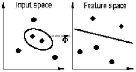
Fig.1 The idea of kernel method

In the FCM algorithm we use the following objective function in eq(2) for minimization. From the equation (2), we can see that classical FCM algorithm is based on the input space sum-of-squares clustering criterion. If the separation boundaries between clusters are nonlinear then FCM will unsatisfactorily work. To solve this problem we adopt the strategy of nonlinearly mapping the input space into a higher dimensional feature space and then performing linear FCM within the feature space. Assume we define the nonlinear map as ,φ: x → φ(x)ϵF where xϵΧ. X denotes the input space, and F denotes the feature space with higher dimension. Note that the cluster centre in the feature space can now be denoted by the following form

vi =∑k=l βik φ(xк)for all i;

where β ik is the coefficients which will be calculated later. So similar to Equation (1) we select the following objective equation to be optimized

Jm =∑i=l ∑k=l uik ‖φ(xк)-∑1=1 β 11 φ(x 1 )‖2 (7)

We rewrite the norm in equation (7) as the following:

‖φ(xк)-∑βil φ(x1)‖

= φ(xк)T φ(xк)-2∑lU β11 φ(xк)т φ(x1)+ ∑ "=1 ∑Г=1 β 11φ(xк)Тβ 1) φ(xj) (8)

It’s interesting to see that equation (2) takes as the form of a series of dot products in feature space. And these dot products can easily be computed through Mercer kernel representations in the input space

K(x, y) =. φ(x) т φ(y)

Thus the equation (8) can be formulated as follows

‖φ(xк)-∑Г=1 β il φ(x1)‖2 =K кк-2βiKк+βi Kβ i

(9a)

where β i = (β il,βi2,…․,βin)T ,і = 1,2,…,c; K = (K kl,Kk2,…,Kkn )T and K = (K ! ,K2,…․․,Kn) for k =1,2,..., n

We can calculate K ij in the following way

Kij=K(xi,xj) for all i,j = 1,2,…,n.

where K is also named the kernel function. While any function satisfying the Mercer condition can be used as the kernel function, the best known is polynomial kernels, radial basis functions and Neural Network type kernels. Substituting for the norm in equation (8) with equation (9a), we get

Jm =∑i=l ∑k=l uik (K kk-2βiKк+βi Kβ i )

Minimizing J m with m > 1 under the constraint of equation (1b), we have the expressions of u ik and β I as follows

(1/(Ккк-грТкк+рТкр!) /()

u ik = ∑ i=i (Kkk-2pTKk+pTKPi) /()

for all i,k;

(10a)

β = ^∑ β= _∑

∑ for all I

(10b)

• D.    Kernelized Type2 fuzzy c-means clustering algorithm

Rhee and Hwang [17] extended the type-1 membership values (i.e. membership values of FCM) to type-2 by assigning a membership function to each membership value of type-1. Their idea is based on the fact that higher membership values should contribute more than smaller memberships values, when updating the cluster centers. Type-2 memberships can be obtained as per following equation:

l-uik aik=uik -

Where aik and uik are the Type-2 and Type-1 fuzzy membership respectively. From (11), the type-2 membership function area can be considered as the uncertainty of the type-1 membership contribution when the center is updated. Substituting (11) for the memberships in the center update equation of the conventional FCM method gives the following equation for updating centers.

^∑Li^(aik^{) m}x_k ^v‘ =_∑k-i(^)

During the cluster center updates, the contribution of a pattern that has low memberships to a given cluster is relatively smaller when using type-2 memberships and the memberships may represent better typicality. Cluster centers that are estimated by type-2 memberships tend to have more desirable locations than cluster centers obtained by type-1 FCM method in the presence of noise. T2FCM algorithm is identical to the type-1 FCM algorithm except equation (12). At each iteration, the cluster center and membership matrix are updated and the algorithm stops when the updated membership and the previous membership i.e. max ik|a new-аfk |< £ , £ is a user defined value. Although T2FCM has proven effective for spherical data, it fails when the data structure of input patterns is non-spherical and complex.

Kernel based extension (KT2FCM)

(KT2FCM) adopts a kernel induced metric which is different from the Euclidean norm in the original Type-2 fuzzy c-means. KT2FCM minimizes the objective function:

JKT2FCM=2∑i=l ∑k=l аik ‖Φ(xк) - Φ(vi)‖2  (13a)

Here aik is the Type-2 membership. Where ‖Φ(xк) - Φ(vi)‖2 is the square of distance between Φ(xк)and Φ(vi).

The distance in the feature space is calculated through the kernel in the input space as follows:

‖Φ(xк) - Φ(vi)‖2

= (Φ(xк) - Φ(vi))․ (Φ(xк) - Φ(vi))

= Φ(xк)․ Φ(xк) - 2Φ(xк)Φ(vi) +Φ(vi)․ Φ(vi)

= K(xк,xк) -2K(xк,vi)+K(vi,vi)           (13b)

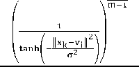
We can use any kernel given in the section A examples. As Hyper Tangent kernel has been used in this technique so:

K(x,y)=1 - tanh (- ^‖ 4 ^‖ ),

Where is σ іs defined as kernel width and it is a positive number, then

K(x, x) = 1

Thus (13a) can be written as

JKT2FCM= 2∑f=l ∑k=l а ik (1 - K(xк,vi))

JKT2FCM =2∑i=l ^∑k=l ^аik (tanh(- ^‖ ^ ^‖ ))       (14)

Theorem 1: The necessary conditions for minimizing J KT2FCM under the constraint of U, we get:

a =

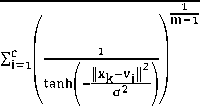
∑k=iaik К(xk, )(1+tanh( ‖ Xk;2Vi ‖ ))Xk

∑ k~, a^K(xk, )(1+tanh(

^‖ ^ ^‖ ))

The optimal values of the kernel width can be obtained through (14),

• E.    Kernelized Intuitionistic fuzzy c-means clustering algorithm

Intuitionistic fuzzy c-means clustering algorithm is based upon intuitionistic fuzzy set theory. Fuzzy set generates only membership function Д( X ), X ∈ X , whereas Intutitionistic fuzzy set (IFS) given by Atanassov considers both membership fi ( x ) and nonmembership V ( X ). An intuitionistic fuzzy set A in X, is written as:

A={x, Ha (x), vA (x)|x∈X}

Where ц_А ( x ) → [0,1], V_A ( x ) →[0,1] are the membership and non-membership degrees of an element in the set A with the condition:

0≤H(x)+Уд (x)≤1.

When V_A ( X )=1- Цд ( X ) for every x in the set A, then the set A becomes a fuzzy set. For all intuitionistic fuzzy sets, Atanassov also indicated a hesitation degree, Пд ( X ), which arises due to lack of knowledge in defining the membership degree of each element x in the set A and is given by:

Лд (X)=1-Ha (x)-vA (x);    0≤лА (x)≤1

Due to hesitation degree, the membership values lie in the interval

[Ha (x), Ha (x)+Лд (x)]

Intuitionistic fuzzy c-means (T. Chaira, 2011)[2] objective function contains two terms: (i) modified objective function of conventional FCM using Intuitionistic fuzzy set and (ii) intuitionistic fuzzy entropy (IFE). IFCM minimizes the objective function as:

JlFCM =∑ 1 = 1 ∑ k=l^{u ∗} ™^ik +∑ i = l^ ^∗e^{1   ∗}      (17)

u∗ =    + ^•ik, where U∗ denotes the intuitionistic fuzzy membership and "^ik denotes the conventional fuzzy membership of the kth data in ithclass.

TC[k is hesitation degree, which is defined as:

^ik =1- ^-tk -(1-Uik“ ) ⁄a,a>0, and is calculated from Yager’s intuitionistic fuzzy complement as under:

N(x) =       (1-x“ ) ⁄a,a>0, thus with the help of Yager’s intuitionistic fuzzy compliment , Intuitionistic Fuzzy Set becomes:

And hesitation degree is given by:

л∗=  ∑k=i^tk,k∈ [1, N]

Second term in the objective function is called intuitionistic fuzzy entropy (IFE). Initially the idea of fuzzy entropy was given by Zadeh in 1262. It is the measure of fuzziness in a fuzzy set. Similarly in the case of IFS, intuitionistic fuzzy entropy gives the amount of vagueness or ambiguity in a set. For intuitionistic fuzzy cases, if M'A ( X_t ), V_A ( X[ ), ^A ( X[ ) are the membership, non-membership, and hesitation degrees of the elements of the set X={ x_r , ■^■2 ,…․․x_n}, then intuitionistic fuzzy entropy, IFE that denotes the degree of intuitionism in fuzzy set, may be given as:

IFE (A)=∑7=1^( Xi )e[ 1-ЛД ( Xi)]                (19)

Where Л_А ( Xi )=1- Ha ( Xi )- V_A ( Xi ).

IFE is introduced in the objective function to maximize the good points in the class. The goal is to minimize the entropy of the histogram of an image.

Modified cluster centers are:

∗ ^∑ к-т ^uik^xk

=∑n u∗ ∑

At each iteration, the cluster center and membership matrix are updated and the algorithm stops when the updated membership and the previous membership i.e.

max_ik | U ^∗ new - u ^∗< |< e , £is a user defined value.

Kernel based extension

The model RBF kernel based Intuitionistic fuzzy c-means (KIFCM) adopts a kernel induced metric which is different from the Euclidean norm in the original intuitionistic fuzzy c-means. KIFCM minimizes the objective function: c n

Ikifcm=2∑∑и∗m ‖Φ(Xk)-Φ(^)‖2

i=l k=l

+∑   Л ^∗ _el-n ∗

^—4 = 1

where ‖Φ( Хк )-Φ(1^)‖² is the square of distance between Φ( Xi ) and Φ( ^к ) and can be calculated as in eq (13b). We can use any kernel given in the section A examples As Radial basis kernel has has been used in this technique so:

∑|X? - ХГ | b_ \

К(х,У)=exp(-         )

Where a and b is greater than 0, and а is defined as kernel width and it is a positive number, then

К(х,х)=1․

Hence,

‖Φ(хк)-Φ(VI)‖2 =2(1-К(хк , V())

Thus (21) can be written as:

Jkifcm =2∑∑ и ^∗ к¹ (1- К ( Хк , Vi )) 1=1 к=1

+∑  л∗е1"" ∗

^-^1=1

Jkifcm =2∑∑и∗т(1-exp(

+∑   И ^∗ е¹"⁷¹ ∗

^—4=1

-

∑| х?

-

а2

X» ^| ))

Given a set of points X, we minimize Jkifcm in order to determine и ^∗ &  ^1 . We adopt an alternating optimization approach to minimize Jkifcm and need the following theorem:

Theorem 1: The necessary conditions for minimizing Jkifcm under the constraint of U, we get:

∗       ^{( (} « (ь, , _{)) )}

=

∑   (( Т. ( 7. , . _{)) )}

∑k=iu∗р×К(Хк, ^ )×Хк Vi=∑к=1и∗к1×К(Хк,vi)

• III. Simulations & Results

In this section, we describe the experimental results on four synthetic images bacteria and hand. There are total of four algorithms used i.e. FCM, KFCM, KIFCM and KT2FCM. Note that the kernel width σ in kernelized methods has a very important effect on performances of the algorithms. However how to choose an appropriate value for the kernel width in kernelized methods is still an open problem. In this project we adopt the “trial and error” for each image for each algorithm and set the parameter σ variably. In addition we set the parameter N (total number of iterations)=200, m=2, ξ=3e-2 in the rest experiments. Experiments are implemented and simulated using

MATLAB Version R2001a and Intel(R) Core(TM) i5 CPU 2.27 GHZ 3GB RAM, 64BIT Operating System.

We test the algorithms’ performance when corrupted by “Gaussian” and “salt and pepper” noises both qualitatively and quantitatively. Qualitative analysis of the algorithms’ is discussed in section III.A and quantitative analysis is discussed in section III.B.

• A.    Qualitative Analysis

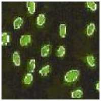
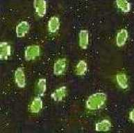
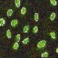
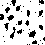
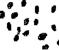
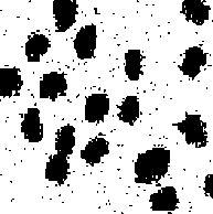
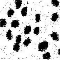
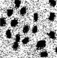
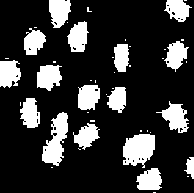
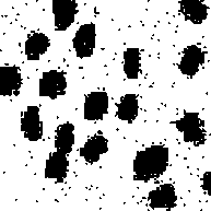
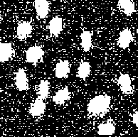
Bacteria Image

Test Image Bacteria (123x123) is generated as shown in fig 1(a). Salt and pepper noise and Gaussian noise of intensity 0.02 is added to generate image 1(b) and (c) respectively. By analyzing the 2nd row fig 1(d), 1(e), 1(f) which is the output when FCM algorithm is applied we observe segmentation is good in all the three cases but by looking at the bacteria we observe that FCM is unable to remove Gaussian or salt and pepper noise. KFCM (fig 1(g), 1(h), 1(i)) shows good segmentation, but we observe that it results in increased size in outputs. Looking at the bacteria we see KFCM removes both the type of noises. KIFCM fig 1(j),1(k), 1(l), as with KFCM it results in increased size in outputs .Results are almost same as KFCM but more noise is removed in case of KFCM . With KT2FCM fig 1(m),1(n),1(o), in case of noiseless segmentation is not very clear on boundaries though its clearer when noise is present.KT2FCM even remove some noise. So in case our image is noiseless FCM and KFCM both show equivalent result so any can be used. While when salt and pepper is present KT2FCM should be used and in case Gaussian is present any of the kernel methods can be used.

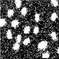
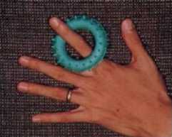
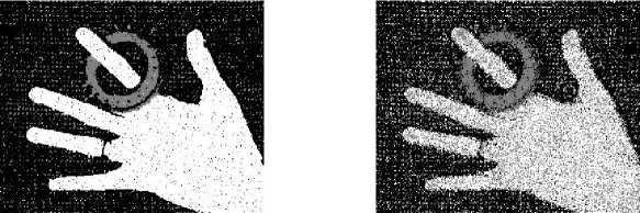
Hand Image

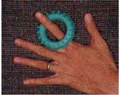
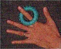
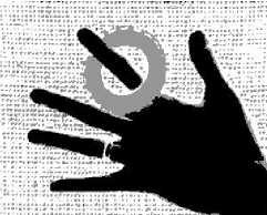
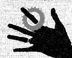
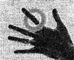
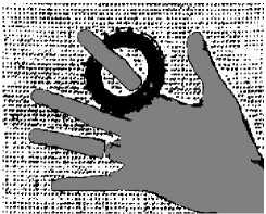
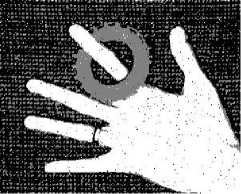
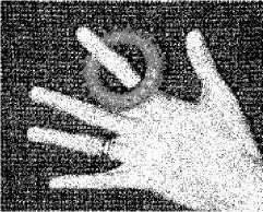
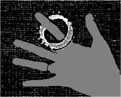
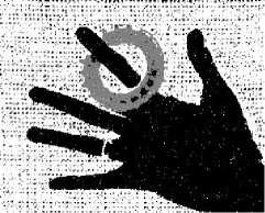
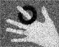
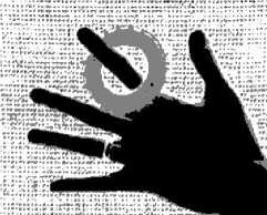
Test Image Hand (303x243) is generated as shown in fig 2(a). Salt and pepper noise and Gaussian noise of intensity 0.02 is added to generate image 2(b) and 2(c) respectively. By analyzing the 2nd row fig 2(d), 2(e), 2(f) which is the output when FCM algorithm is applied we observe good performance in all the three cases, though best as expected with noiseless. FCM shows better performance with salt n pepper as compared to with Gaussian. FCM is unable to remove Gaussian noise. Moving to result of KFCM (fig 2(g), 2(h), 2(i)) we observe that KFCM shows its best performance with salt n pepper. It almost removes salt n pepper. Performance with noiseless is also good. In case of Gaussian noise it succeeds in marginally reducing the noise but segmentation of some portion of ring not clear. Analysing output of KIFCM fig 2(j), 2(k), 2(l), segmentation is not proper with noiseless and salt n pepper as ring area not properly detected. Segmentation is better with Gaussian but unable to remove Gaussian noise or even salt n pepper. With KT2FCM fig 2(m), 2(n), 2(o) best segmentation as compared with other algorithms is observed. KT2FCM even removes salt and pepper and Gaussian to some extent. So we can say that if noiseless case then, undoubtedly FCM is best and very near to it is KT2FCM. With KIFCM and KFCM segmentation not good with the ring part. In case its salt and pepper then KFCM is the winner. KT2FCM removes some noise but fails in ring segmentation. For Gaussian there is a close fight among all the algorithms. While KFCM removes some noise, segmentation is not that good in the ring part. While segmentation is best with KIFCM, noise not at all removed.

• B.    Quantitative Analysis

Based on Execution Time

Bacteria Image

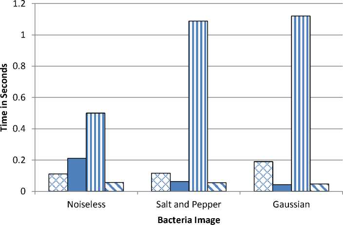
Fig 3 shows the bar chart of the execution time of FCM,KFCM,KIFCM and KT2FCM for Bacteria Image in three different case of noiseless, salt and pepper and Gaussian. FCM performs best with noiseless and worst with Gaussian. While it is seen that KFCM performs best with Gaussian and worst with salt and pepper. KIFCM has max execution time with Gaussian and least with noiseless. KT2FCM least execution time as compared to other algorithm. It shows almost same time in all the three cases. Hence KFCM andKT2FCM show best execution time while KIFCM the worst performance.

Hand Image

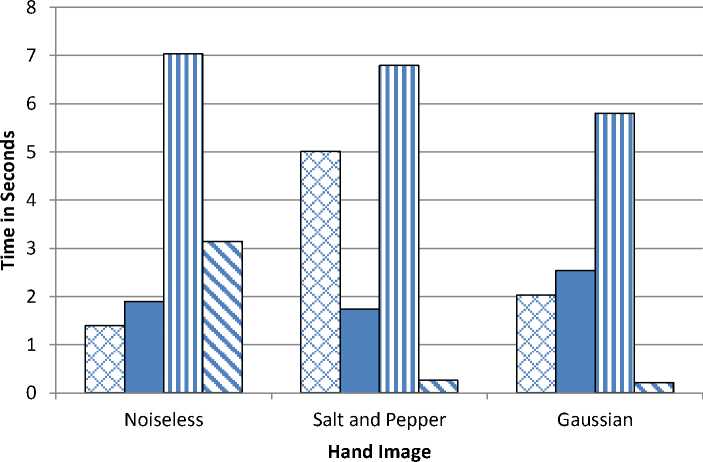
Fig 4 shows the bar chart of the execution time of FCM,KFCM,KIFCM and KT2FCM for Hand Image in three different case of noiseless, salt and pepper and Gaussian. In FCM we observe least execution time with noiseless and maximum with salt and pepper. With KFCM best performance with salt and pepper and worst with Gaussian. In case its KIFCM we see large execution time as compared to other algorithms. KIFCM shows best in Gaussian and worst as expected with noiseless.KT2FCM shows least execution time as compared to other algorithms. Best with Gaussian and worst in salt and pepper. Based on execution time we can say , KIFCM has worst performance while KT2FCM shows best.

(a)

(b)

(c)

(d)

(e)

(f)

f

(g)

(h)

(i)

(j)

(k)

(l)

(m)

(n)

(o)

• Fig.1: Ouputs on bacteria image Column 1 shows output of algorithms in noiseless case, column 2 shows output in salt and pepper noise and cloumn 3 shows output with gaussian noise.

Fig 1(a),1(b),1(c) are the original images in the 3 cases of noiseless,salt and pepper, and gaussian respectively.

Fig 1(d), 1(e), 1(f) represents output of FCM in the 3 cases.

Fig 1(g),1(h),1(i) represents output of KFCM in the 3 cases.

Fig 1(j),1(k),1(l) represents output of KIFCM in the 3 cases.

Fig 1(m),1(n),(o) represents output of K2FCM in the 3 cases.

(a)

(b)

(c)

(d)

(e)

(f)

(g)

(h)

(i)

(j)

(k)

(l)

(m)

(n)                                          (o)

Fig. 2: Ouputs on hand image Column 1 shows output of algorithms in noiseless case, column 2 shows output in salt and pepper noise and cloumn 3 shows output with gaussian noise.

Fig 2(a),2(b),2(c) are the original images in the 3 cases of noiseless,salt and pepper, and gaussian respectively.

Fig 2(d), 2(e), 2(f) represents output of FCM in the 3 cases.

Fig 2(g),2(h),2(i) represents output of KFCM in the 3 cases.

Fig 2(j),2(k),2(l) represents output of KIFCM in the 3 cases.

Fig 2(m),2(n),2(o) represents output of K2FCM in the 3 cases.

о FCM

• □    KFCM

• □    KIFCM

и K2FCM

• Fig. 3:    Bar Chart of Bacteria Image

  
  
  

  и FCM

  
  

  □ KFCM

  
  

  □ KIFCM

  
  

  □ K2FCM

  
  

• Fig. 4:    Bar Chart of Hand Image

• IV. Conclusion

In this paper we have discussed the performance of the four algorithms FCM, KFCM, KIFCM, KT2FCM for the synthetic digital images in noiseless case and when corrupted with salt and pepper and Gaussian noise. We compare these algorithms both qualitatively i.e. segmentation evaluation and quantitatively i.e. based on execution time and validity function. Based on segmentation evaluation we can say that FCM dominates when it comes to noiseless case closely followed by KFCM. In case noise is present kernel methods show better performance if compared with FCM. Among the kernel methods KFCM seems to be the best followed by close fight between KT2FCM and KIFCM depending on the input image. Analyzing based on execution time and comparing the results of all the four images, we can say FCM executes in smallest time. Comparing the kernel methods we can conclude that KIFCM takes the maximum time while KFCM and KT2FCM the least. Also as expected time to execute is lesser with two clusters than with three clusters.The results reported in the project show that kernel method is an effective approach to constructing a robust image clustering algorithm. This method can also be used to improve the performance of other FCM like algorithms based on adding some penalty terms to the original FCM objective function.