RLS Wiener Smoother for Colored Observation Noise with Relation to Innovation Theory in Linear Discrete-Time Stochastic Systems

Published Online February 2013 in MECS DOI: 10.5815/ijitcs.2013.03.01

In comparison with the Kalman estimators, the RLS Wiener estimators are advantageous in the point that the RLS Wiener estimators do not use the information of the input noise variance and the input matrix in the state equation for the signal. The less information in the estimators might avoid the degradation of the estimation accuracy caused by the inaccurate information on the state-space model. In [1], the RLS Wiener filter and fixed-point smoother are proposed in linear discretetime stochastic systems. The estimators need the information of the system matrix, the observation vector, the variance of the state vector and the variance of white observation noise. In addition, in linear discretetime stochastic systems, the following RLS Wiener estimators are studied, i.e. the Chandrasekhar-type RLS Wiener fixed-point smoother, filter and predictor [2], the square-root RLS Wiener fixed-point smoother and filter [3] and the RLS Wiener FIR filter [4], etc.

Almost estimators are designed for the white observation noise. In the estimation problems, there might be actual cases where the observation noise is colored. The estimation problem for the observation equation, with additive colored observation noise, has received much attention in the detection and estimation problems for communication systems. For example, in [5]-[10], the estimation problem is considered in linear discrete-time stochastic systems. In [8], an alternative method is proposed on the traditional handling of the autoregressive colored observation noise in the speech enhancement algorithm based on the Kalman filter. In [10], based on the autoregressive moving average (ARMA) innovation model, the reduced-order Wiener estimators for descriptor system with MA colored observation noise and multi-observation lags are presented.

In [11], for the white observation noise, the signal estimation problem is considered in linear continuoustime stochastic systems. Also, the spectral factorization method is discussed on the system matrix, the input matrix and the observation matrix. That is, the innovation state-space model for the colored observation model is developed.

In [12], based on the improved least-squares (ILS) method, the parameter estimation technique for a noisy autoregressive (AR) signal, observed with additive colored noise, is presented.

In [13], starting with the Wiener-Hopf equation, the RLS Wiener fixed-point smoother and filter are presented for the colored observation noise. By the way, the innovation theory is an interesting method, which has been investigated in the area of the estimation techniques for the white observation noise. It might be worthwhile to consider the RLS Wiener smoothing problem also for the colored observation noise. This paper, with the relation of the work in [13] to the innovation theory [14], [15], newly proposes the discrete-time smoother for the colored observation noise in linear wide-sense stationary stochastic systems. It is assumed that the smoothing estimate is given as a linear transformation of the innovation process. The approach, adopted in this paper, to the design of the RLS Wiener smoother has not be examined hitherto in the case of the colored observation noise. Based on the RLS Wiener smoother, the fixed-interval smoothing algorithm for the colored observation noise is shown in the flowchart of Fig.1. The observation y(k) is given as a sum of the signal z(k) = Hx(k) and the colored observation noise v (k) . The RLS Wiener estimators use the following information: (a) the system matrix for the state vector x(k) ; (b) the observation matrix H ; (c) the variance of the state vector; (d) the system matrix for the colored observation noise v (k) ; (e) the variance of the colored observation noise; (f) the input noise variance in the state equation for the colored observation noise. Also, the filtering error variance function P~ (L,L) and the prediction error variance function ~(L, L -1) , for the signal z (L) , are formulated with regard to the current RLS Wiener estimators.

In section 2, the smoothing problem, based on the innovation theory, is introduced. In section 3, Theorem 1 proposes the RLS Wiener smoothing and filtering algorithms. In section 4, Fig. 1 depicts the flowchart for the fixed-interval smoothing estimate z ˆ( k , L ) .

A numerical simulation example, in section 4, shows the estimation characteristics of the proposed RLS Wiener fixed-interval smoother and filter for the colored observation noise.

• II.    Least-Squares Smoothing Problem Based on Innovation Theory

Let m-dimensional observation equation be described by y (k) = z (k) + vc (k), z (k) = Hx (k)       (1)

in linear discrete-time stochastic systems. Here, H is an m x n observation matrix, z ( k ) is the zero-mean signal vector. The process { _v= ( k ), k > 0} represents the zero-mean colored observation noise sequence. It is assumed that the signal is uncorrelated with the colored observation noise as

E [ z ( k ) V T ( 5 )] = 0 , 0 <  k , 5 < w .          (2)

Let K ( k , ₅ ) = K ( k - ₅ ) represent the auto-covariance function of the state vector x ( k ) in wide-sense stationary stochastic systems [16], and let K ( k , s ) be expressed in the form of

K x ( k , s )

Г A ( k ) B T ( 5 ),

t B ( 5 ) A^T ( k ),

0 <  5 <  k ,

0 <  k <  5 ,

A ( k ) = Ф ^k ,   B T ( 5 ) = Ф^{- 5}K_x ( 5 , 5 ).

Here, Ф is the transition matrix of _x ( k ).

Let the state-space model for x(k) be described as x (k +1) = Фx (k) + Gw (k),

E[w(k)wT (5)] = Q(k)3K (k - 5), where G is an n x l input matrix and w(k) is the white input noise vector with the auto-covariance function of (4).

Let K ( - , - ) denote the auto-covariance function of v ( k ) . The auto-covariance function K ( k , s ) is given by

K (k, 5) =j Ac (k) BT (5),  0 < 5 < k, c         [ Bc (5) AT (t),   0 < k < 5,

A c ( k ) =Ф k ,   B c ^T ( 5 ) = Ф - K ( 5 , 5 ).

Let the state equation for v ( k ) be given by

V c ( k + 1) = Ф c V c ( k ) + u ( k ),

E[u (k)uT (5)] = Ru (k)5K (k - 5), in terms of the white input noise vector u(k) with the variance R . It is found that for the expressions Kc (k +1, k +1) = E [ vc (k +1) vcT (k +1)], K (k, k) = E[vc (k)vj(k)], in the wide-sense stationary stochastic systems, the following relationships hold.

R u ( k ) = K c ( k + 1, k + 1) - Ф c K c ( k , k ) Ф T , K c ( k + 1, k + 1) = K c ( k , k ) = K c (0)

It is shown that the fixed-interval smoothing estimate x ˆ( k , L ) of x ( k ) is given by

LL

:v ( k , L ) = ^ g ( k , i ) u ( i ) = x ( k , k ) + ^ g ( k , i ) u ( i ), i = 1                                        i = k + 1

x( k , k ) = ]T g ( k , i ) u ( i ) i = 1

in terms of the impulse response function g ( k , i ) and the innovation process { y ( i ), 1 <  i <  L } [14], [15]. Also, x ˆ( k , k ) represents the filtering estimate of x ( k ) , which is given as a linear transform of the innovation process { u ( i ), 1 <  i <  k } .

Let us consider the estimation problem, which minimizes the mean-square value (MSV)

J = E [|| x ( k ) - x( k , L )||²]                  (9)

of the fixed-point smoothing error x ( k ) - x ( k , L ) . From an orthogonal projection lemma [16],

x ( k ) - ∑ ^L g ( k , i ) υ ( i ) ⊥ υ ( s ),  1 ≤ s ≤ L ,   (10)

i = 1

the impulse response function satisfies the equation

E [ x ( k ) υ ^T ( s )] = ∑ ^L g ( k , i ) E [ υ ( i ) υ ^T ( s )].   (11)

i = 1

Here ‘ ⊥ ’ denotes the notation of the orthogonality. From [13], the filtering estimate xˆ(k, k) of x(k) is calculated sequentially by xˆ(k, k) = Φxˆ(k-1, k-1) +G(k)(y(k)

- ( H Φ x ˆ( k - 1, k - 1) + ( Φ )² v ˆ ( k - 1, k - 1) (12)

+Φ v ˆ ( k - 1, k - 1))),   x ˆ(0,0) = 0.

It is clear that the innovation process υ(k) is expressed as

υ ( k ) = y ( k ) -( H Φ x ˆ( k -1, k -1) +Φ c ² v ˆ 2 ( k -1, k -1)+Φ c v ˆ 3 ( k -1, k -1)).

Also, from (8) and (12), the filter gain G ( k ) is equivalent to g ( k , k ) . For the innovation process satisfying

E [ υ ( k ) υ^T ( s )] = ∆( k ) δ ( k - s ), (14)

from (11), the impulse response function g ( k , s ) and the filter gain G ( k ) are given by

g ( k , s ) = E [ x ( k ) υ^T ( s )]∆^-1( s ), G ₁( k ) = g ( k , k ). (15)

From [13], it is seen that the variance Δ( L ) of the innovation process { υ ( L ), L ≥ 0} is formulated as (29) in Theorem 1.

• III.    RLS Wiener Smoothing Equations

Under the linear least-squares estimation problem of the signal z ( k ) in section 2, Theorem 1 presents the RLS Wiener smoothing and filtering equations, which use the covariance information of the signal and the observation noise.

• Theorem 1

Let the auto-covariance function K ( k , s ) of the state vector x ( k ) be expressed by (3), let the variance of the colored observation noise v ( k ) be K ( k , k ) and let the variance of u ( k ) in the state equation (6) for v ( k + 1) be R ( k ) . Then, the discrete-time RLS Wiener algorithms for the smoothing estimate and the filtering estimate of the signal z ( k ) consist of (16)-(45) in linear wide-sense stationary stochastic systems.

Smoothing estimate of the signal z ( k ): z ˆ( k , L )

zˆ(k, L) =Hxˆ(k, L)

Smoothing estimate of x ( k ) : x ˆ( k , L )

xˆ(k, L) = xˆ(k,k)+ f0(k+1,L)- f1(k+1,L)

- f 2 ( k +1, L )- f 3 ( k +1, L ))

f 0 ( k +1, L )= f 0 ( k +1, L -1)

+K (k,k)(ΦT)L-kHTΔ-1(L)υ(L), f (k+1,k+1)=K (k, k)ΦTHTΔ-1(k+1)υ(k+1)

f 1 ( k +1, L )= f 1 ( k +1, L -1)+( d 1 ^T ( k , L -1)

+dT(k+1,L-1))HT∆-1(L)υ(L), f (k+1,k+1)=ST(k)ΦTHTΔ-1(k+1)υ(k+1)

f 2 ( k +1, L )= f 2 ( k +1, L -1)+( d 3 ^T ( k , L -1)

+dT(k+1,L-1))∆-1(L)υ(L), f (k+1,k+1) =ST(k)(ΦT)2Δ-1(k+1)υ(k+1)

f 3 ( k +1, L )= f 3 ( k +1, L -1)+( d 5 ^T ( k , L -1)

+dT(k+1, L-1))∆-1(L)υ(L), f (k+1,k+1) =ST(k)ΦTΔ-1(k+1)υ(k+1)

d ( k , L )=Φ d ( k , L -1)-Φ G ( L )( Hd ( k , L -1)

+d (k,L-1)+d (k, L-1)), d (k, k) = ΦS (k)

d ( k +1, L )=Φ d ( k +1, L -1)

+ΦG (L)(HΦL-kK (k,k) -Hd (k+1,L-1)

-d (k+1,L-1)-d (k+1,L-1)), d (k+1,k+1)=ΦG (k+1)HΦK (k,k)

d ( k , L )=Φ d ( k , L -1)

-Φ2G (L)(Hd (k,L-1)+d (k,L-1)

+d5(k,L-1)), d3 (k,k) = Φc2S21 (k)

d 4 ( k +1, L )=Φ c d 4 ( k +1, L -1)

+ Φ c ² G 2 ( L )( H Φ ^{L - k}K x ( k , k )

- Hd ( k +1, L -1)- d ( k +1, L -1)

-d6(k +1,L-1)), d (k+1,k+1) =Φ2G (k +1)HΦK (k,k)

d ( k , L ) = Φ d ( k , L -1)

-Φ c G 3 ( L )( Hd 1 ( k , L -1)+ d 3 ( k , L -1)          (26)

+d5(k,L-1)), d5(k,k) = ΦcS31(k)

d 6 ( k +1, L )=Φ c d 6 ( k +1, L -1)

+ Φ c G 3 ( L )( H Φ ^{L - k}K x ( k , k )

- Hd ( k +1, L -1) - d ( k +1, L -1)

• - d 6 ( k +1, L -1)),

d ( k +1, k +1)=Φ G ( k + 1) H Φ K ( k , k )

Innovation process: y(L )

^u( L ) = y ⁽ L ) - ^{( H} ® x ⁽ L - 1, L - 1)                (28)

+ Ф 2 v ₂( L - 1, L - 1) + Ф _cv ₃ ( L - 1, L - 1)).

Variance of the innovation process y ( L ): A( L )

A( L ) = R u ( L ) + ( HK x ( L , L ) - ( H Ф 5 „ ( L - 1)Ф ^T

+ (Ф c )² 5 21 ( L -1)Ф ^T +Ф c 5 31 ( L - 1)Ф ^T )) H^T

+ (Ф c K c ( L , L ) - ( H Ф 5 1 ₂( L -1)Ф c              ⁽²9)

+ (Ф c )² 5 22 ( L - 1)Ф c + Ф c 5 32 ( L - 1)Ф c ))Ф c

+ ( R u ( L ) - ( H Ф 5 1з ( L -1)Ф c

+ (Ф c ) 2 5 23 ( L - 1)Ф c + Ф c 5 33 ( L - 1)Ф T )).

Filtering estimate of the signal z ( L ) : z ˆ( L , L )

z ( L , L ) = Hx ( L , L )                              (30)

Filtering estimate of x ( L ) : x ˆ( L , L )

x ( L , L ) = Ф x ( L -1, L -1) + G_x ( L )( y ( L)

• -    ( H Ф x ( L -1, L -1) + (Ф _c )² v ₂( L -1, L -1)     ⁽³¹⁾

+ Ф Л ( L -1, L -1))),   x (0,0) = 0

Filtering estimate of v ( L ) :

Ф c v 2 ( L , L ) + v ( L , L ))

V ( L , L ) = Ф c v 2 ( L -1, L -1) + G 2 ( L )( y ( L )

• -    ( H Ф x ( L -1, L -1) + (Ф_с)² v ₂ ( L -1, L -1)     ⁽³²⁾

+ Ф _cv ₃( L -1, L -1))),   v 2 (0,0) = 0

V ( L , L ) = Ф c v 3 ( L -1, L -1) + G з ( L )( y ( L )

• -    ( H Ф x ( L -1, L -1) + (Ф _c )² v ₂ ( L -1, L -1)     (33)

+ Ф Л( L -1, L -1))),

• V (0,0) = 0

Filtering variance function of x ˆ( L , L ) : S ( L )

5 _u( L ) = E [ x ( L , L ) x ^T ( L , L )]

• 5 _п( L ) = Ф 5 _п( L -1)Ф ^T

+ G , ( L )( HK_X ( L , L ) - ( H Ф 5 _п( L - 1)Ф ^T      (34)

+ (Ф c )² 5 21 ( L - 1)Ф ^T + Ф c.5 31 ( L - 1)Ф ^T )),

• 5 „(0) = 0

Cross-variance function of x ˆ( L , L ) with v ˆ ( L , L ) : 5 12 ( L ) = E [ ; x ( L , L ) V 2 ^T ( L , L )]

5 12 ( L ) = Ф 5 12 ( L -1)Ф T

+ G 1 ( L )(Ф c K c ( L , L ) - ( H Ф 5 12 ( L - 1)Ф T           (35)

+ (Ф c . )² 5 22 ( L - 1)Ф T +Ф c 5 32 ( L - 1)Ф T )),

5 12 (0) = 0

Cross-variance function of x ˆ( L , L ) with v ˆ ( L , L ) : 5 1з ( L ) = E [ x ( L , L ) v^T₃ ( L , L )]

5 1з ( L ) = Ф 5 1з ( L -1)Ф T + G 1 ( L )( R u ( L )

• -    ( H Ф 5 1з ( L -1)Ф T + (Ф c . )² 5 2з ( L -1)Ф T         ⁽³⁶⁾

+ Ф c S зз ( L - 1)Ф ^T _c )),   5 13 (0) = 0

5 21 ( L ) = Ф c 5 21 ( L - 1)Ф ^T + G 2 ( L )( HK x ( L , L )

• -    ( H Ф 5 11 ( L - 1)Ф ^T + (Ф c )² 5 21 ( L - 1)Ф ^T          (37)

+ Ф c. 5 31 ( L -1)Ф ^T )),   5 21 (0) = 0,

5 21 ( L ) = 5 T 2 ( L )

Filtering variance function of v ˆ ( L , L ) : S ( L )

5 22 ( L ) = Ф c. 5 22 ( L -1)Ф T

+ G 2 ( L )(Ф c K c ( L , L ) - ( H Ф 5 12 ( L - 1)Ф T         (38)

+ (Ф c . )² 5 22 ( L - 1)Ф T + Ф c. 5 32 ( L - 1)Ф T )),

5 22 (0) = 0

Cross-variance function of v ˆ ( L , L ) with v ˆ ( L , L ) : 5 2з ( L ) = E [ V ( L , L ) V^T ( L , L )]

5 2з ( L ) = Ф c 5 2з ( L -1)Ф T

+ G 2 ( L )( R u ( L ) - ( H Ф 5 1з ( L - 1)Ф T               (39)

+ (Ф c . )² 5 23 ( L - 1)Ф T + Ф c. 5 33 ( L - 1)Ф T )),

5 23 (0) = 0

5 31 ( L ) = Ф c. 5 31 ( L - 1)Ф ^T + G з ( L )( HK x ( L , L )

• -    ( H Ф 5 11 ( L - 1)Ф ^T + (Ф _c )² 5 ₂₁ ( L - 1)Ф ^T         (40)

+ Ф c.5 31 ( L - 1)Ф ^T )),   5 31 (0) = 0,

5 31 ( L ) = 5 T 3 ( L )

5 32 ( L ) = Ф c 5 32 ( L - 1)Ф T

+ G з ( L )(Ф c K c ( L , L ) - ( H Ф 5 12 ( L - 1)Ф c

+ (Ф c )² 5 ₂₂( L - 1)Ф T +Ф c 5 32 ( L - 1)Ф T )),

5 32 (0) = 0,

5 32 ( L ) = 5 ₂ ^Г з ( L )

Filtering variance function of v ˆ ( L , L ) :

5 зз ( L ) = E [ V ( L , L ) V 3 ^T ( L , L )]

5 зз ( L ) = Ф c. 5 зз ( L - 1)Ф T

+ G з ( L )( R u ( L ) - ( H Ф 5 1з ( L - 1)Ф T              (42)

+ (Ф c . )² 5 23 ( L - 1)Ф T + Ф c. 5 33 ( L - 1)Ф T )),

5 зз (0) = 0

Filter gain for x ˆ( L , L ) : G ( L )

G i (L ) = [ K x ( L , L ) H T -Ф 5 _n( L -1)Ф T H T -Ф 5 12 ( L -1)(Ф TT )² -Ф 5 1з ( L -1)Ф T ] x [ R u ( L ) + ( HK x ( L , L ) - ( H Ф 5 „( L - 1)Ф T + (Ф _с )² 5 21 ( L -1)Ф T +Ф _С5 31 ( L - 1)Ф T )) H T + (Ф _сK c ( L , L ) - ( H Ф 5 12 ( L -1)Ф C + (Ф с )² 5 22 ( L - 1)Ф c + Ф с 5 32 ( L - 1)Ф c ))Ф c + ( R u ( L ) - ( H Ф 5 1з ( L -1)Ф c

+ (Ф c )² 5 23 ( L - 1)Ф c +Ф c 5 33 ( L - 1)Ф c ))]^-1

fixed-interval smoothing algorithm, a numerical example is demonstrated. The fixed-interval smoothing estimate is calculated according to the flowchart in Fig. 1.

Let a scalar observation equation be described by

У ⁽ k ) = ^{z ( k} ) ⁺ v c ⁽ k )   z ( k ) = Hx ( k )

Filter gain for v ˆ₂ ( L , L ) : G ( L )

G 2 ( L ) = [ K c ( L , L )Ф T - Ф c 5 21 ( L - 1)Ф T H T

-Ф c S ₂₂( L - 1)(Ф С )² -Ф c S 23 ( L - 1)Ф T ]

x [ R u ( L ) + ( HK x ( L , L ) - ( H Ф 5 _u( L - 1)Ф ^T

+ (Ф c )² 5 21 ( L - 1)Ф ^T +Ф c 5 31 ( L - 1)Ф ^T )) H^T     (  )

+ (Ф c K c ( L , L ) - ( H Ф 5 ₁₂( L - 1)Ф c

+ (Ф c )² 5 ₂₂ ( L - 1)Ф T + Ф c 5 32 ( L - 1)Ф I ))Ф I

+ ( R u ( L ) - ( H Ф 5 _B( L - 1)Ф I

+ (Ф c )² 5 23 ( L - 1)Ф I + Ф c 5 33 ( L - 1)Ф I ))]^-1

Filter gain for v ˆ ( L , L ): G ( L )

Here, ^{v c ( k )} is the zero-mean colored observation noise. Let the signal ^{z ( k )} be generated by the second-order AR model.

z ( k +1) = - a_xz ( k ) - a₂z ( k -1) + w ( k ), E [ w ( k ) w ( s )] = c r² ^ ( k - s ), a, =-0.1,   a ₂ =-0.8, c = 0.5.

The corresponding state-space model for ^{z ( k )} can be written as

z ( k ) = Hx ( k ) = x _] ( k ),   H = [ 1  0 ],   x ( k ) =

x 1 ( k + 1)	=	" 0	1 "	x 1 ( k )	+	"0"	w ( k ).
_ x 2 ( k + 1) .		- а 2	- а^	_ x 2 ( k ) .		.1.

x X k ) x ₂( k )J,

G 3 ( L ) = [ R u ( L ) -Ф c 5 31 ( L -1)Ф ^T H^T -Ф c 5 32 ( L - 1)(Ф c )² - Ф c 5 33 ( L - 1)Ф I ] x [ R u ( L ) + ( HK x ( L , L ) - ( H Ф 5 „ ( L - 1)Ф ^T + (Ф c )² 5 21 ( L - 1)Ф ^T + Ф c 5 31 ( L - 1)Ф ^T )) H^T + (Ф c K c ( L , L ) - ( H Ф 5 12 ( L - 1)Ф ^Tc

+ (Ф c )² 5 22 ( L - 1)Ф I +Ф c 5 32 ( L - 1)Ф I ))Ф I + ( R u ( L ) - ( H Ф 5 13 ( L -1)Ф f

+ (Ф c )² 5 23 ( L - 1)Ф I + Ф c 5 33 ( L - 1)Ф I ))| '

The auto-covariance function of the signal ^{z ( k )} is

described as follows [13]:

K (0) = c ²,

k ( m ) = c ²{ a ( a 2 - 1)0 " /[( a - a )( aa +1)] - a ( a ² - 1) a m /[( a - a )( aa +1)]},

0 <  m , a , a = (- ^a i ± 4^а 2 -4 ^a 2 )/2.

From (49) and (50), it can be found that

Proof of Theorem 1 is deferred to the Appendix.

From Theorem 1 , the filtering error variance function P ^~ ( L , L ) and the prediction error variance function j~,( L , L - 1), for the signal z ( L ), are given by

K x ( k , k )

K (0) K (1)

K (1) 1       Г 0

K (0)],  ° = [- a₂

K (0) = 0.25,   K (1) = 0.125.

—

a

P~ f ( L , L ) = K_z ( L , L ) - H5 ₁₁( L ) H T ,                (46)

j° ( L , L -1) = K ( L , L ) - H Ф 5 j ( L - 1)Ф T H T .

Let the state equation for ^{v c ( k )} be given by

V c ( k +1) = Ф c V c ( k ) + u ( k ),

E [ u ( k ) u^T ( s )] = R„5_K ( k - s ),

Ф _c = 0.91,   R u = 0.01,

where K ( L , L ) represents the variance function of the signal z ( L ).

According to the smoothing and filtering algorithms in Theorem 1 , the calculation steps for the fixed-interval smoothing estimate z ˆ( k , L ) of the signal z ( k ) can be shown in the flowchart of Fig. 1.

where ^{u ( k )} is the white input noise in the state equation (52) for the colored observation noise process. The autovariance function of the colored observation

IV. A Numerical Simulation Example

In this section, to show the efficiency of the estimation characteristics of the proposed RLS Wiener

noise      v^c        satisfies     the     relationships

K ( k + 1, k + 1) = K ( k , k ) = K (0)    . ,       .,■  .   . .

^{c      ,           c ,        c} and hence, this lead to

Kc (0) = R^^

^{1 - a} in wide-sense stationary stochastic

systems.

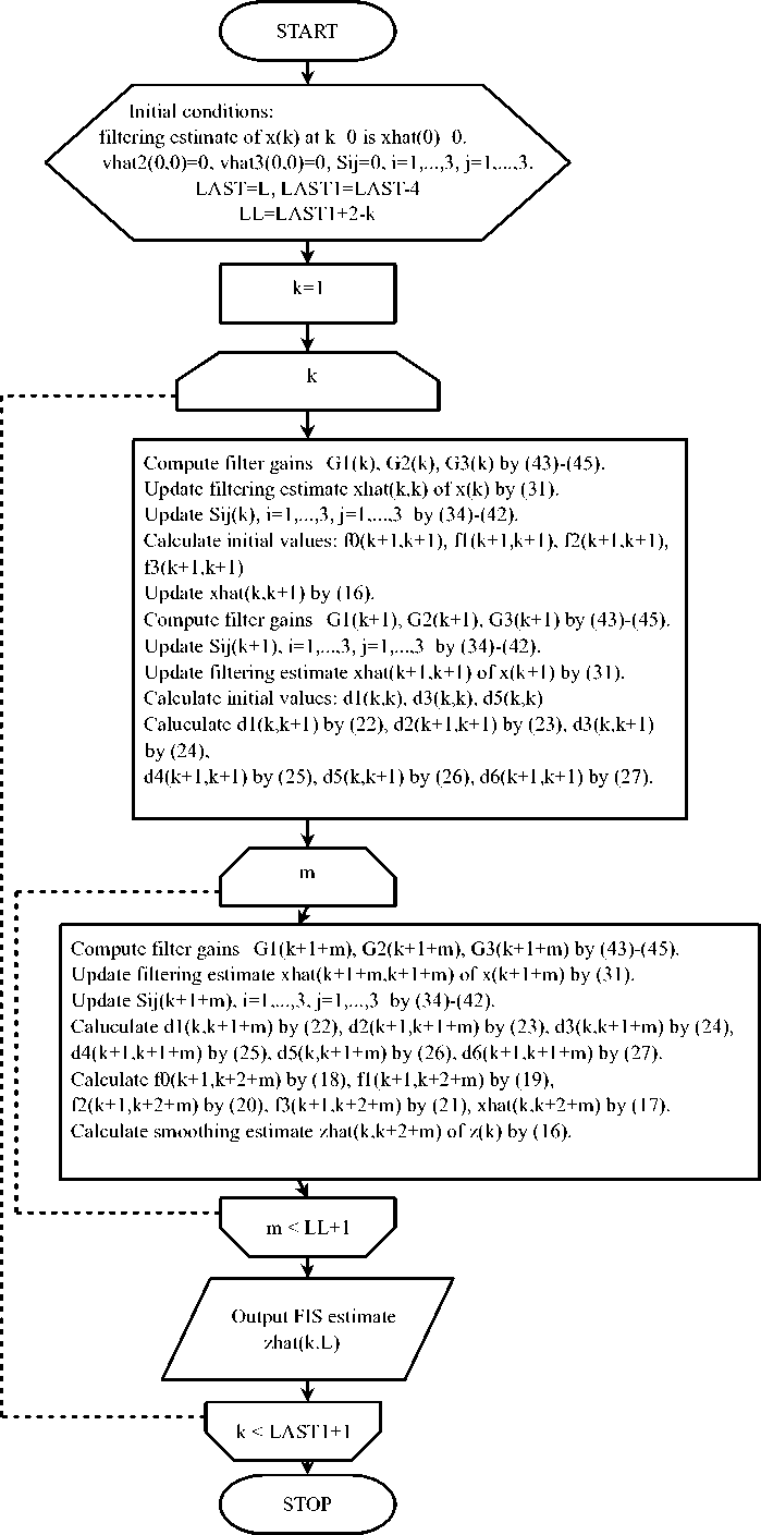
Fig. 1: Flowchart for the fixed-interval smoothing estimate z ˆ( k , L ) .

Substituting H , Φ , ^K x ^{( L , L ) = K} x ⁽⁰⁾ , ^Φ c , ^{K c ( L , L )= K c (0)} and ^{R u} into the RLS Wiener estimation algorithms of Theorem 1 , the fixed-interval smoothing and filtering estimates are calculated.

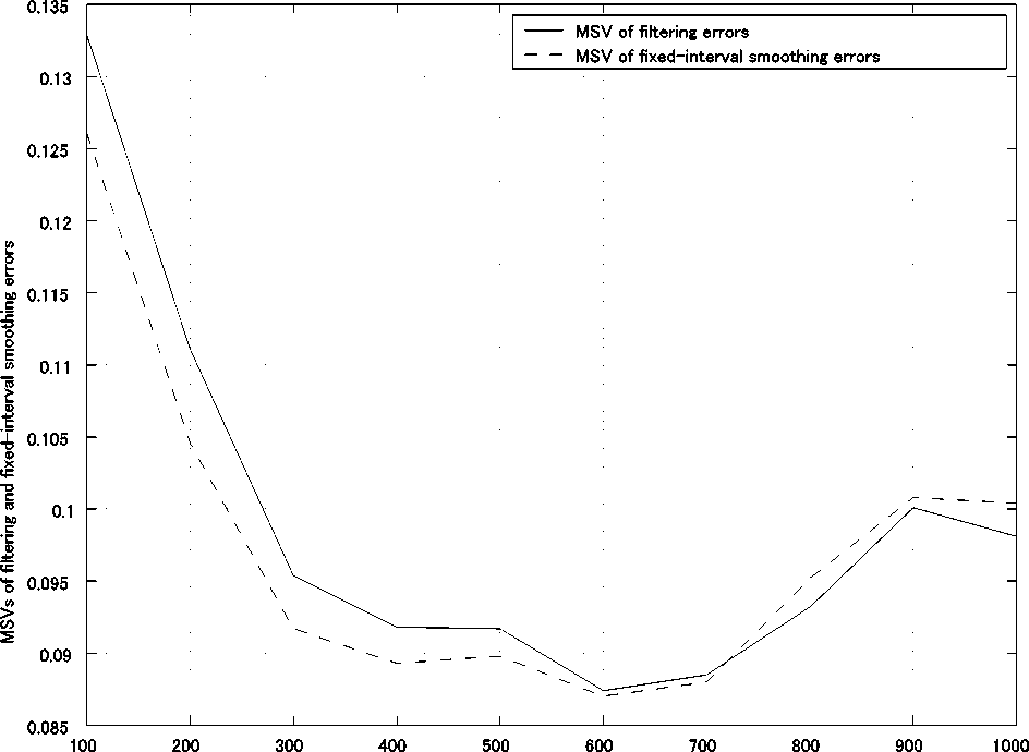
Fig. 2 illustrates the colored observation noise process ^{v c ( k )} vs. ^k , ^{1 ≤ k ≤ 500} , for the variance ^{R u = 0.01} in (52). Fig. 3 illustrates the fixed-interval smoothing estimate ^{z ˆ( k , L )} , ^{L = 500} , vs. ^k , ^{1 ≤ k ≤ 500} , for the variance ^{R u = 0.01} . Fig. 4 illustrates the MSVs of the filtering errors ^{z ( L ) - z ˆ( L , L )} of the signal ^{z ( L )} and the fixed-interval smoothing errors ^{z ( k ) - z ˆ( k , L )} of

^{z ( k )} vs. vs. L for ^R u ^{=0.001( K} c ^(0)=0.0582) . In Fig. 4, as the fixed interval ^L increases, ^{100 ≤ L ≤ 600} , the MSV of the fixed-interval smoothing errors gradually decreases. Also, for ^{100 ≤ L ≤ 700} , the MSV of the fixed-interval smoothing errors ^{z ( k ) - z ˆ( k , L )} is less than the MSV of the filtering errors ^{z ( k ) - z ˆ( k , k )} , ^{1 ≤ k ≤ L} . Hence, the estimation accuracy of the fixed-interval smoother is better than that of the filter for ^{100 ≤ L ≤ 700.} From this fact, the fixed-interval smoothing algorithm, calculated based on the flowchart of Fig. 1, is correct.

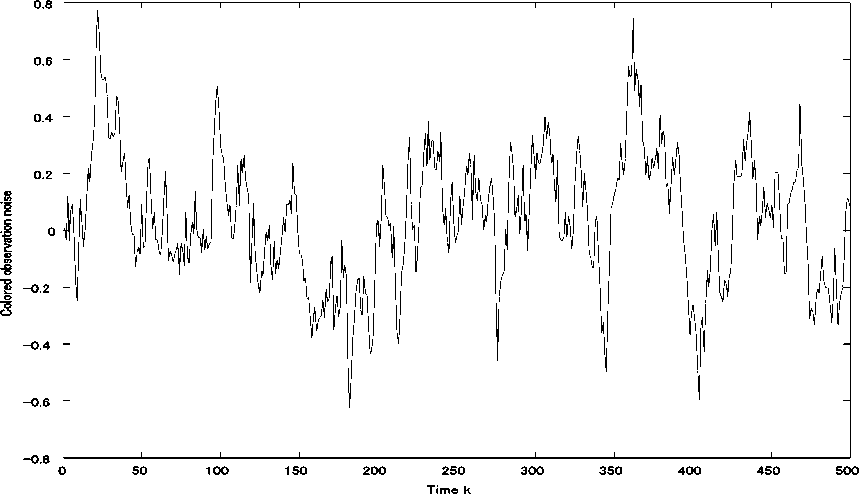
Fig. 2: Colored observation noise process v ( k ) vs. k , 1 ≤ k ≤ 500 , for the variance R = 0.01 in (52).

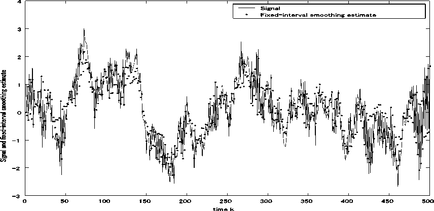
Fig. 3: Fixed-interval smoothing estimate z ˆ( k , L ) , L = 500 , vs. k for the variance R = 0.01 .

Fixed interval L

Fig. 4: MSVs of the filtering errors z ( k ) - z ˆ( k , k ) , 1 ≤ k ≤ L and the fixed-interval smoothing errors z ( k ) - z ˆ( k , L ) vs. L , 100 ≤ L ≤ 1000 .

• V. Conclusions

In this paper, the RLS Wiener smoothing problems, with relation to the innovation theory, have been considered for the colored observation noise.

A numerical simulation example has shown that the proposed estimation algorithms for the RLS Wiener fixed-interval smoothing and filtering estimates, in the case of the colored observation noise, are feasible. In Fig. 4, as the fixed interval L increases, 100 ≤ L ≤ 600 , the MSV of the fixed-interval smoothing errors gradually decreases. Similar tendency, on the estimation accuracy, also fit to the RLS Wiener filter. Also, for 100 ≤ L ≤ 700, the MSV of the fixed-interval smoothing errors z ( k ) - z ˆ( k , L ) is less than the MSV of the filtering errors z ( k ) - z ˆ( k , k ), 1≤ k ≤ L . Hence, for 100≤ L ≤700, the estimation accuracy of the RLS Wiener fixed-interval smoother is superior to that of the RLS Wiener filter for the colored observation noise.

The RLS Wiener estimators do not use the information of the variance Q(k) , for the input noise w(k) , and the input matrix G in the state equation (4), in comparison with the Kalman estimation technique [13]. In the RLS Wiener estimators, it is not necessary to take account of the degraded estimation accuracy caused by the modeling errors for Q(k) and G .