Robust monocular visual odometry trajectory estimation in urban environments

Published Online October 2019 in MECS

In the past years, inertial sensors, odometry were used with GPS sensors for estimating location in case of GPS blackout [3, 4]. With odometry sensors, the vision-based method displayed to be very accurate and effective in the position estimation and the orientation of the autonomous vehicle [11]. Visual odometry (VO), referred to an egomotion estimation, is an essential capability that determines the trajectory of a moving robot in its environment based on estimate camera motion connected to the robot [1]. However, the image itself is a matrix of brightness and color, and it would be very difficult to consider motion estimation directly from the matrix level. Therefore, we are accustomed to adopting such an approach: First, select a more representative point from the image. These points will remain the same after a small change in camera angle, so we will find the same point in each image. Then, based on these points, the problem of camera pose estimation and the positioning of these points are discussed [2]. With the large-spread use of cameras in different fields of robotics, there has been a revolution in algorithms of visual odometry with a wide-set of aspects including monocular VO [13], stereo VO [14, 15]. In this context, it has been shown that visual odometry provides more precise estimation than other mechanics; furthermore, today the digital cameras are accurate, compact, and inexpensive.

Although stereo VO system can provide very accurate estimation, using two or more cameras require complex mechanistic support for complex hardware and software equipment and the cameras for parallel image elaboration and acquisition; this increases the cost and the complexity of the overall system when compared to the systems of simple mono-camera. Thus, it is important the improvement of reliable mono-camera based VO algorithms to be utilized in low-cost trajectory estimation frameworks.

The accuracy and reliability of visual odometry estimation depend also on the selection of the medium frames to be applied for relative motion estimate along the trajectory. The frames are typically obtained at a constant rate and every monocular pose of the camera is retrieved by immediately matching the present frame to the previous frame. Furthermore, it can be possible that using different sets of matching frames extracted over the path, can have a spectacular effect on the precision of trajectory rebuilding. In this context, it is important the determination of efficient metrics and methodologies for the selection, on-line, of the most reliable frames to be employed for an accurate trajectory rebuilding.

This study focuses on the visual mileage calculation method based on the feature point method , we will divide our work into several steps, extract and match image feature points, and then estimate the camera motion and scene structure between the two frames to achieve a basic two-frame visual odometer and then at final determine the trajectory of a moving robot. In addition, this proposed algorithm is shown to output reliable robust Monocular visual odometry even for longer paths of several kilometers.

The feature point consists of Key-point and Descriptor. The key point refers to the position of the feature point in the image, and some feature points also have information such as orientation, size. A descriptor is usually a vector that describes the information about the pixels around the key in a way that is artificially designed. The descriptors have been designed according to the principle that "features with similar appearance should have similar descriptors".

The Structure of the paper as the following. The next section (II) reviews the related work. Section (III) gives details of Feature points and feature matching. Section (IV) describes the Triangulation. Section (V) explains the PnP method and its equations. Section (VI) describes experimental and results, with summarized conclusions described in Section VII.

• II.    Related Work

In the last decades, various forms of the equations of motion equations have been introduced, and the solution method based on nonlinear optimization has been explained [1]. RANSAC was used for 3D to 2D camera pose estimation and outlier rejection to compute the new camera pose [1]. The object features were used over a long time window and a large part of the display area was for object projection. The systems that use the motion models smoothed the camera trajectory and constrain the search space for feature across frames. Chiuso et al. He introduced the latest approach in this class and presented an inverse depth in the case vector, thus converting the equation of nonlinear measurement into an identity [12].

Estimating a vehicle’s ego-motion from input based on camera alone has been started in the eighties and was explained by Moravec. The most of the previous researches in Visual Odometry were done for planetary was driven by the NASA exploration program in the effort to supply rovers with the high capability to measure their 6-degree of freedom (6 DoF) motion in all terrains [2, 12].

In the area of pedestrian navigation, the Pedestrian Dead-Reckoning methodologies have been inspected for urban localization [7, 6]. The pose is incrementally specified by calculating the displacement between poses after the initial public pose is obtained with other methodologies like appearance-based localization. Sensor fusion is an alternate method and has also been inspected to recompense for the drawback of each sensor [8, 5]. The fusion was shown to compensate for shortcomings in appearance-based methodologies because of failure under quick rotational motions. IMU has two important units, a gyroscope, and an accelerometer. A gyroscope has a characteristic that it can precisely route sensor angular rates for short time periods. An accelerometer is useful through the static stage to estimate global orientation by using the gravity measurement [8].

Structure from motion (SFM) problem in the computer vision society has been deeply studied in the past years and it was employed for recovering poses from a collection of images [4]. In the robotics community, Simultaneous Localization and Mapping (SLAM) is the problem closely identified with the structure from motion problem. SLAM is the contemporaneous estimate of the robot movement and the simultaneously constructing and updating of the environmental map [9].

Our new method differs from previous approaches through the introduction of artificially designed feature points and provides highly accurate trajectory estimates, reducing the time of extraction of key points and the calculation of descriptors. Additionally, this method can be integrated into other visual odometry methods.

• III.    Feature Points

Feature points represent some special points in the image. “Fig. 1,” We regard the corners, edges, and blocks in the image as representative places in the image. Note that the corners and edges in the image are more "special" than the pixel blocks, and can be distinguished between different images. Therefore, an intuitive way to extract features is to identify corner points between different images and determine their correspondence. In this approach, corner points are so-called features.

The ORB (Oriented FAST and Rotated BRIEF) feature is a very representative real-time image feature. It improves the problem that the FAST detector [11] is not directional, and uses the extremely fast binary descriptor BRIEF [12] to greatly accelerate the entire image feature extraction.

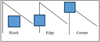
Fig.1. A figure shows part of image features: corners, edges, and blocks.

• A.    Fast

FAST is a kind of corner point, which mainly detects the obvious change of gray level of local pixels, and is known for its fast speed. The idea is that if a pixel differs greatly from the pixels in its neighborhood (too bright or too dark), it is more likely to be a corner. Compared to other corner detection algorithms, FAST only needs to compare the brightness of pixels, which is very fast. Its detection process is as follows “ Fig.2.”.

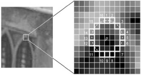
Fig.2. A figure shows FAST detection process [18].

Select the pixel P in the image, assuming its brightness is Ip, Set a threshold T (such as 20% of Ip), Center the pixel p and select 16 pixels on a circle with a radius of 3, If the brightness of consecutive N points on the selected circle is greater than Ip + T or less than Ip - T, then pixel p can be considered as a feature point (N is usually taken as 12, which is FAST-12. Another commonly used N is 9 and 11, which are called FAST-9, FAST-11), Loop through the above four steps to perform the same operation for each pixel.

• B.    Brief

After extracting the Oriented FAST key points, we calculate their descriptors for each point. BRIEF is a binary descriptor whose description vector consists of a number of 0s and 1s, where 0 and 1 encode the size relationship of two pixels near the key (such as p and q): if p is greater than q, then take 1 and vice versa. So how do we choose p and q? In general, the positions of p and q are randomly chosen according to a certain probability distribution. BRIEF uses randomly selected points for comparison, which is very fast, and because of the use of binary expression, it is also very convenient to store, which is suitable for real-time image matching [19].

The original BRIEF descriptor has no rotation invariance, so it is easy to lose when the image rotates. ORB calculates the direction of key points in FAST feature point extraction stage, so we can use the direction information to calculate the "Steer BRIEF" feature after rotation, so that the descriptor of ORB has better rotation invariance.

• C.    Feature matching

Feature matching refers to find corresponding features based on two analogous datasets based on a specific search distance. One of these datasets is considered as source and the other one is target, especially when we use the feature matching to derive rubber-sheet links. By accurately matching the descriptor between image and image, or between image and map, we can reduce a lot of burden for subsequent attitude estimation, optimization and other operations.

Consider an image of two moments. If feature points x^m , m = 1, 2... M are extracted from image It, and feature points xⁿ , n = 1, 2... N are extracted from image It+1, then we need to find the corresponding relationship between these two set elements. The simplest feature matching method is Brute-Force Matcher. That is, for each feature point x^m , the distances of the descriptors are measured with all xⁿ , and then sorted, taking the nearest one as the matching point. The descriptor distance represents the similarity between the two features. For descriptors of floating point type, Euclidean distance is used to measure them. For binary descriptors (such as BRIEF), we often use Hamming distance as a measure -the Hamming distance between two binary strings, referring to the number of different digits “Fig. 3”.

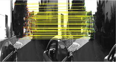
Fig.3. A figure shows Feature matching between two frames.

• IV.    Triangulation

In the previous sections, we estimated the camera motion. After getting the motion, the next step is to estimate the spatial position of the feature points with the motion of the camera. In monocular VO, the depth information of the pixels cannot be obtained only from a single image. We need to estimate the depth of the map points by triangulation.

Triangulation means that the distance of the point is determined by observing the angle of the same point at two locations. Triangulation was first proposed by Gauss and applied in surveying, it has been used in astronomy and geographic surveys. For example, we can estimate the distance of a star from us by observing its angle in different seasons. In VO, we mainly use triangulation to estimate the distance of pixels.

Similar to the previous section, consider images I1 and I2, take the left image as a reference, and the transformation matrix of the right image as T. The camera's optical centers are O1 and O2. There is a feature point p1 in I1, and a feature point p2 in I2. In theory, the straight lines O1p1 and O2p2 intersect in the scene at a point P, which is the position of the map points corresponding to the two feature points in the threedimensional scene. According to the definition in polar geometry, let X1 and X2 be the normalized coordinates of two feature points, then they satisfy:

5₁х₁ = sRx + t               (1)

Now we already know R, t, what we want to solve is the depth of two feature points S1, S2. Of course, these two depths can be separated. Let's look at S2 first. If we want to count S2, then first multiply the left side of the above formula by x^1 to get:

S j X f X j = 0 = s₂x ^f Rx₂ + x f t (2)

• V.    Pnp

PnP (Perspective-n-Point) is a method for solving 3D to 2D point pair motion. It describes how to estimate the pose of a camera when we know n 3D spatial points and their projected positions. The 3D position of feature points can be triangulated or determined by the depth map of RGB-D camera. In a monocular visual odometer, initialization must be performed before PnP can be used. 3D-2D method is the most important attitude estimation method, which does not need polar constraints and can obtain better motion estimation at very few matching points. [10].

• A. P3P

P3P needs to utilize the geometric relationship of three given points. Its input data are three pairs of 3D-2D matching points. Note that the 3D points are A, B, C, and 2D points are a, b, C. where the lowercase letters represent the projection of uppercase letters on the imaging plane of the camera, as shown in “Fig. 4,”. In addition, P3P also needs to use a pair of verification points to select the correct one from the possible solutions.

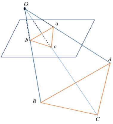
Fig.4. A figure shows Schematic diagram of P3P problem

The verification point pair is D_d and the camera's optical center is O. Note that we know the coordinates of A, B, C in the world coordinate system, not in the camera coordinate system. Once the coordinates of 3D point in the camera coordinate system can be calculated, we can get the corresponding points of 3D-3D and transform PnP problem into ICP problem.

Firstly, it is obvious that there are corresponding relations between triangles:

Aoab - AOAB, Aobc - AOBC, Aoac - AOAC (3)

Consider the relationship between oab and OAB. Using the cosine theorem, there are:

OA2 + OB2 - 2OA • OB • cos(a, b) = AB2

For the other two triangles, there are similar properties, so there are:

OB2 + OC2 - 2OB • OC • cos (b, c) = BC2

OA2 + OC2 - 2OA • OC • cos (a, c) = AC2

Divide all three formulas above by OC2, and remember x = OA/OC, y = OB/OC, to get:

X2 + y2 - 2xy cos (a, b) = AB2/OC2

Y2 + I2 - 2y cos (b, c) = BC2/OC2

X2 + I2 - 2x cos (a, c) = AC2/OC2

Remember v =AB2/OC2, uv = BC2/OC2, wv = AC2/OC2, with:

X2 + y2 - 2xy cos (a, b) - v= 0

Y2 + I2 - 2y cos (b, c) -uv = 0

X2 + I2 - 2x cos (a, c) - wv= 0

We can put V in the first formula on the side of the equation and substitute the second and third equations to get:

(1 - u) y2 - ux2 - cos(b, c)y+ 2uxycos(a, b) +1 = 0

(1 - w) x 2 - wy2 - cos (a, c) x + 2wxy cos (a, b) + 1 = 0

Notice the known and unknown quantities in these equations. Since we know the image position of 2D points, three cosine angles cos (a, b), cos (b, c), cos (a, c) are known. At the same time, u=BC2/AB2, w = AC2/AB2 can be calculated by the coordinates of A, B, C in the world coordinate system, after transformation to the camera coordinate system, this ratio does not change. The x,y in this formula are unknown and will change as the camera moves. Therefore, this system of equations is a binary quadratic equation concerning x,y. Similar to the case of decomposition E, the equation can obtain up to four solutions, but we can use verification points to calculate the most probable solution and get the 3D coordinates of A, B, C in the camera coordinate system. In order to solve PnP, we use the triangle similarity property to solve the 3D coordinates of projection points a, b, C in the camera coordinate system. Finally, we transform the problem into a 3D to 3D pose estimation problem.

• VI.    Experimental Results

In this section, the proposed Monocular VO method was evaluated by using two outdoor scenes: sequences 00 and 12 from the public KITTI VO benchmark [17]. Sequences 00 is collected with the accurate ground truth, sequence 12 is provided only with the raw sensor without ground truth. Table 1. summarises the sequences of KITTI which were used.

Table 1. Kitti Sequences Datasets [17].

Sequence	#Images	Image size (Px)	Dist(Km)
00	4541	1241x376	3.73
12	1061	1226x370	1.23

The experimental environment platform for this paper as shown in Table 2.

Table 2. Details of the experimental platform.

Details of the test platform.
Processor	Intel Core i7 CPU @ 3.40 GHz 3.40 GHz
OS	Ubuntu 16.04
Memory	8GB RAM
SW Env.	C++, MATLAB R2018a

Firstly, ORB features have been extracted and matched, we do this part by calling several mainstream image features which have been integrated with OpenCV. Fig.6.

shows the results of this process. Next, we want to estimate the camera's motion based on these matched pair of points. When computing ORB on a set of 4541 images with 1241x376 px, it was able to detect and compute over 2×108 features in 40 seconds.

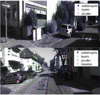
Fig.5. A figure shows p3p and triangulation process, the up one displays the first stage of initializing candidate key points and p3p before triangulation, the down one displays the triangulation stage

Based on the Images pose which solved based on p3p, we find the spatial position of this feature point by triangulation, we call the triangulation function provided by OpenCV to triangulate. “Fig. 5,” Shows p3p and triangulation process, the up one displays the first stage of initializing candidate key points and p3p before triangulation, the down one displays the triangulation stage. The 3D-points can be rebuilt by two views triangulation through features extraction and tracking. Moreover, bundle adjustment is also utilized to refine the 3D-reconstruction. For robust estimation, ORB (Oriented FAST and Rotated BRIEF) and PnP (Perspective-n-Point) are used to help against outliers.

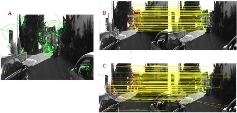
Fig.6. A figure shows Feature extraction and matching results, A). ORB Key Points, B). Filtered matching, C). Unfiltered matches.

Note that in “Fig. 7,” the estimated trajectory was well aligned together with the ground truth, The blue line is estimated trajectory and the dotted black line is the actual trajectory based on ground truth, this aligned was kept the same from the start to the end except at some places where it is well aligned with the street as shown in “Fig.8,”.

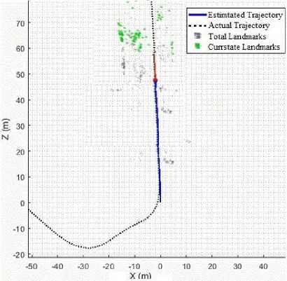
Fig.7. A figure shows the estimated trajectory was well aligned together with the ground truth.

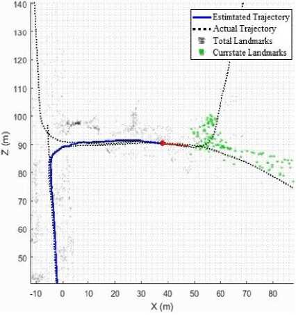
Fig.8. A figure shows the estimated trajectory was aligned with the street.

• VII.    Conclusion

In this paper, ORB and PnP method was applied to provide accuracy trajectory estimation. The proposed method combines the key points, which has been extracted from ORB (Oriented FAST and Rotated BRIEF) and Feature matching. This proposed method is evaluated by using the longest two sequences 00 and 12 from public KITTI dataset. This proposed algorithm provides a highly accurate trajectory estimates, with very small relative position error. Experiments show promised results in accurate trajectory estimation where it success to extract the distinguished key points which improve Monocular VO performance. Our proposed approach is inexpensive computationally and can be adapted easily with most Monocular VO algorithms depending on feature tracking. Finally, image sequences from public KITTI dataset have been used to verify the robustness and high performance of our proposed method.

Acknowledgment

We thank the Software Engineering Laboratory of the school of Information Engineering at the China University of Geoscience (Wuhan) for materials and intellectual support during this work.