Rough Set Model for Nutrition Management in Site Specific Rice Growing Areas

Author: K. Lavanya, N.Ch.S.N. Iyengar, M.A. Saleem Durai, T. Raguchander
Journal: International Journal of Intelligent Systems and Applications(IJISA) @ijisa
Article in issue: 10 vol.6, 2014.
Free access
The optimized fertilizer usage for better yield of rice cultivation is influenced by key factors like soil fertility, crop variety, duration, season, nutrient content of the fertilizer, time of application etc., It is observed that 60 percent of yield gap in tamilnadu is due to farmers lack of knowledge on key factors and informal sources of information by pesticide dealers. In this study the major contributing factors for fertilizer requirement and optimum crop yield were analyzed based on rough set theory. In data analytics perspective the nutrient plan is sort of multiple attribute decision-making processes. To reduce the complexity of decision making, key factors that are indiscernible to conclusion are eliminated. Our rough set based approach improved the quality of agricultural data through removal of missing and redundant attributes. After pretreatment the data formed as target information, then attribute reduction algorithm was used to derive rules. The generated rules were used to structure the nutrition management decision-making. The precision was above 88% and experiments proved the feasibility of the developed decision support system for nutrient management.
Rough Set, Attribute Reduction, NPK Supplies
Short address: https://sciup.org/15010618
IDR: 15010618
Text of the scientific article Rough Set Model for Nutrition Management in Site Specific Rice Growing Areas
-
I. Introduction
Indian paddy cultivation generates a direct or indirect economic livelihood for over 75% of the population .In tamilnadu, rice acreage cultivation is about 19.057 lakh hectares (Directorate of Rice Development, 2010-11). The average yield of rice is about 3040 kg/ha. The suitable season for cost-effective cultivation is kahrif and rabi . The general fertilizer recommendation for irrigated crops is 150-50-50 kg NPK/ha and blanket recommendation for rain-fed crops is 50:25:25 kg NPK/ha (Department of Agriculture, 2012). However most of the farmers in irrigated areas apply excessive amount of fertilizer especially nitrogen fertilizer of 175200 kg N/ha [2] which is considerably higher than the government recommendation. This unwanted investment plays vital role for the yield gap, degradation of soil fertility and post harvest loss.
The growth and development of fertilizer optimization [3] lead to acquisition of numerous key features and its storage in databases. Considering the entire features may slow down the learning process and may reduce the performance of the classifier because of redundant and irrelevant features. Many methods were proposed to mine rules for the growing data. Most of the tools of knowledge mining are crisp, traditional, deterministic and precise in notion. Real situations are very often the reverse of it. The detailed description of the real system needs detailed data which is beyond recognition of the human interpretation. This invoked an extension of the concept of crisp sets to model imprecise, mixed type, incomplete data and enables their modeling intellects.
Rough set theory proposed by pawlak in 1982, is used to study [5] mixed types of data such as continuous, valued and symbolic data. It acts as a knowledge discovery tool that helps to induce logical patterns hidden in massive data. It combines both qualitative and quantitative data in decision making. Rough set analyzes attributes with real values and categorizes the attribute’s value into intervals. These categorical data are subjected to attribute reduction and rule generation [7] that can be used for both key factors selection and knowledge discovery. It helps us to find out the minimal rule sets called reducts to classify objects without deterioration of classification quality and induce minimal length decision rules inherent in the given information system.
In our study, the supporting factors for paddy cultivation are selected from the collected data as conditional attributes and the amount of N, P, K(Nitrogen, Potassium, Sodium) supplies is considered as the decision attribute. As preprocessing these attribute values are mapped on to domain values and coded as numerical (eg. low (1), medium (2), high (3)). Then the lower and upper approximations of elementary sets (the set of objects with the same decision attribute value) are computed. With the help of the proposed algorithm, decision rules are generated by attribute reduction and iterations. Then the decision rules are validated against the threshold value and formulated as a base for nutrition management. Thus we make an attempt to analyze the supporting growth factors and formalize the approximate N,P,K supplement values needed for site specific crops.
The structure of paper is organized as follows. Section II, III highlights the background and basic study respectively. Proposed System is presented in Section IV and evaluation of the proposed system is discussed in Section VI.
-
II. Related Works
Various methodologies used for knowledge discovery are reviewed in this section. The rule reduction [11] can be treated effectively by means of learning premises generalized by genetic algorithm (GA) rather than enumerating AND-connection of input fuzzy sets . The computational efficiency of minimum reducts [12] is highly improved by counting the distinct rows of the subdecision table, instead of generating discernibility functions or the positive regions. The use of entropy in fuzzy-rough feature selection can result in smaller subset sizes than those obtained through FRFS [15] alone, with little loss or even an increase in overall classification accuracy. The Genetic programming [16] is used to construct new features of the data that gives consideration to hide relationships between features. The Particle swarms find optimal regions of the complex search space through the interaction of individuals in the population. PSO is attractive [17] for feature selection and discovers best feature combinations as they fly within the subset space . A new feature called maximum information compression index is generic in nature and has the capability of multi scale representation of data sets. The superiority of the algorithm in terms of speed and performance is established extensively over various real-life data sets of different sizes and dimensions. It is also demonstrated how redundancy [18] and information loss in feature selection can be quantified with an entropy measure . α -Torrent rough set theory is applied to the field of remote sensing classification. The classifier can adapt to the spatial date with severe overlapped features. The experiments results are compared with PCA and traditional rough set[21] this method produces usefully features and improved classification accuracy. The fuzzy rules increase deals with the data pairs contain noise or outlier. The Fuzzy-rough feature selection is introduced for fuzzy rules reduction. To achieve good performance [22] the parameters of fuzzy predictor of every fuzzy rule will be adjusted by learning algorithm. Three novel feature selection techniques employing fuzzy entropy to locate fuzzy-rough reducts is applied. This approach is compared with two other fuzzy-rough feature selection [23] approaches which utilize other measures for the selection of subsets. A rough set reduction scheme for Support Vector Machine (SVM) is used for the classification task [24] based on the significance of each feature vector, while the rough set is applied to improve feature selection and data reduction.
-
III. Basic Concepts Of Rough Set Theory
-
A. Rough Set
Rough set is a formal approximation [1] of a crisp set (i.e., conventional set) in terms of a pair of sets which give the lower and the upper approximation of the original set.
-
B. Information System
Given (U, A) be an information system where U be the finite non empty set (universe) of objects and A is nonempty finite set of attributes (features, variables).For every a ε A, Va is the set of values attribute a may take, called domain of attribute A.
In addition every attribute a ε A defines an information function, D a : U→V
From table 1,
U={x1,x2,x3,x4,x5,x6………….x10}
A={a1,a2,d}
The domains of attributes are
V1 (for a1) = {1,2}
V2 (for a2) = {1,2,3}
V3 (for d) = {1,2}
Table 1. Coded Information Table
|
U |
a1 |
a2 |
d |
|
X1 |
1 |
1 |
2 |
|
X2 |
1 |
2 |
1 |
|
X3 |
1 |
3 |
1 |
|
X4 |
2 |
1 |
2 |
|
X5 |
2 |
2 |
2 |
|
X6 |
2 |
3 |
1 |
|
X7 |
2 |
2 |
1 |
|
X8 |
2 |
3 |
2 |
-
C. Indiscernibility Relation
Two objects x i , x j are said to be indiscernible by their set of attributes B where B ε A, if b(x i ) = b(x j ) ie., every element in the subset B must be equal. It is generally represented as Ind(B). Every subset in Ind(B) is known as elementary set in B because it is the smallest indiscernible group of objects
Table 2. Equivalence Classes
|
U/A |
a1 |
a2 |
|
{x5,x7} |
2 |
2 |
|
{x6,x8} |
2 |
3 |
|
{x1} |
1 |
1 |
|
{x2} |
1 |
2 |
|
{x3} |
1 |
3 |
|
{x4} |
2 |
1 |
Each row in the table 2 represents an elementary set for the information system studied. U/A represents the elementary sets in space A {a1, a2} ie. For instance we are interested in two attributes only.
-
D. Lower and Upper Approximations
For data analysis rough set approach defines two basic concepts namely the lower and the upper approximations of a set. The lower approximation of the set X is a set of objects x i , belonging to the elementary sets contained in X (of space R)
RX = L{Y∈U/R:Y⊆X}
The upper approximation is the union of elementary sets with a non empty intersection to X.
RX = U{Y∈U/R:YA X ≠ φ}
The R–boundary of X , BN ( X ) is given by BN ( X ) = RX - R X . We say x is rough with respect to R if and only if RX ≠ R X , equivalently BN ( Χ ) ≠ φ . X is said to be R – definable if and only if RX = R X or BN ( X ) = φ . So, a set is rough with respect to R if and only if it is not R – definable
Table 3. Discernibility Matrix
|
U |
X1 |
X2 |
X3 |
X4 |
X5 |
X6 |
X7 |
|
X2 |
a2 |
||||||
|
X3 |
a2 |
a2 |
|||||
|
X4 |
a1 |
a1,a2 |
a1,a2 |
||||
|
X5 |
a1 |
a1 |
a1,a2 |
a2 |
|||
|
X6 |
a2 |
a1,a2 |
a1 |
a2 |
a2 |
||
|
X7 |
a1,a2 |
a1 |
a1,a2 |
a2 |
d |
a2 |
|
|
X8 |
a1,a2 |
a1,a2 |
a1 |
a2 |
a2 |
d |
a2 |
-
E. Accuracy of approximation
For the attributes P ⊆Α , we can measure accuracy for any set X ⊆ U ( i.e. α ( X ) ) called the accuracy of approximation as follows:
α Α ( X ) =
cardinality of ΑX cardinality of ΑX
Α X
Α X
Where |X| denotes the cardinality of Obviously
If α B ( X ) = 1 X is crisp with respect to A.
If α ( X ) < 1 X is rough with respect to A
-
F. Independence of attributes
-
G. Attribute Reduction and Rule Deduction
A Decision table is comprised of a set of conditional attributes A and set of decision attributes D.
-
1) . D-Superflous attributes
To find all possible minimal subsets of attributes, leading to a similar number of elementary sets as the whole set of attributes is reduct. To find the set of all dispensable attributes is core. To compute reduct and core the discernibility matrix is used of dimension p x p, where p is the no of elementary sets and its elements are the set of all attributes which discern elementary sets x i and x j
-
2) . D-core and D-Reduct
The set of all D -indispensable attributes in A is called the D -core of A , whereas, the minimal subsets of condition attributes that discern all equivalence classes of the relation Ind( D) discernable by the entire set of attributes are called D -reducts. D-Core and D-reduct aims at removing unnecessary attributes in the decision table.
-
3) . R-core and R-reduct of attributes
The R-reduct uses considerably modified discernibility matrix. An element of the D -discernibility matrix of A is defined as the set of all attributes which discern the objects x i and x j , which do not belong to the same equivalence class of the relation Ind( D) , i.e., to the same class. The D- core is the set of all single elements of the D -discernibility matrix of A . D.Decision Rules deduction
The described decision table can also be regarded as a set of decision classification rules of the form a k i → d j , which means that attribute ‘a k ’ (value ‘i’) leads to decision d (value ‘j’) and ‘→’ denotes propositional implication.
Table 4 . Decision Matrix
|
U |
a1 |
a2 |
d |
|
X1 |
1 |
* |
2 |
|
X2 |
1 |
2 |
1 |
|
X3 |
1 |
* |
1 |
|
X4 |
* |
1 |
2 |
|
X5 |
* |
2 |
2 |
|
X6 |
* |
3 |
1 |
|
X7 |
* |
2 |
1 |
|
X8 |
2 |
3 |
2 |
I(P)=I(P-{a})
If an attribute (a) removal does not increase the number of basic elementary sets then it is a superfluous attribute. Else, attribute (a) is indispensable in space P.
Ind(A)=Ind(A-a1)
The elementary sets after Ind(A-a1) are {{x1,x4},{x2,x7},{x3,x6},{x5},{x8}} which are not same as basic elementary sets so attribute a1 is indispensable in A.
-
IV. Proposed Model
The nutrient plan is sort of multiple attributes decisionmaking processes [9]. It is certain that we have to deal with massive data. Current technologies convert large volume of data into knowledge and use that knowledge to make a proper decision. However, it fails in many instances because the imprecise, uncertain information in the databases are not processed. Rough set theory describes and models the ill-defined data using indiscernibility relation without transforming the data. Our approach uses rough set to deal with complicated attribute aspects such as its importance, interrelations, dimensionality and varied patterns to acquire knowledge directly from data. This work utilizes rough set theory as a preprocessing step to reduce the redundant key factors and to improve the quality of knowledge content in data set. The resultant reduced rule sets from the algorithm serves as a knowledge database for rice nutrition management in site specific regions.

Fig. 1. Rough set based nutrition management
Algorithm
Input:
D,a dataset consisting of training tuples and associated target values
Attr ={c, d}, set of attributes and possible values c:set of conditional attributes;
d:set of decision attributes min_sup: minimum support threshold
-
1 .For each tuple in D
-
2. Divide data in Training and Testing data
-
3. In Training data, construct discernibility matrix and reducts
-
4. While (support of reduct >= min_sup)
-
5. Validation
Repeat
End For
Perform attribute reduction and generate candidate rules
End While
The candidate rules are compared with every object in testing data set. The performance of every rule is computed by
Sum of supported rules pointing to decision d Accuracy=
Sum of supported and non - supported rules
If
Accuracy exceeds min_sup conclude the validated rules as finalized rules
Else
Delete the rule
-
V. Rough Set Methodology-An Illustrative Example
Our study considers a target dataset of 32 elements. To ensure consistency and completeness unreliable and unrelated data were removed to avoid complexity. Data is described in terms of eight attributes based on problem domain. The attributes presented are of two types conditional attributes (a1…a8) and decision attribute (d). Using training dataset candidate rules are generated and are validated against testing dataset using support count and threshold.
Table 5. Target Data Set
Table 6. Reduct And Core [First Iteration]
|
Rules |
a 1 |
a 2 |
a 3 |
a 4 |
a 5 |
a 7 |
a 8 |
d |
Supporting Objects |
|
[1] |
x |
x |
x |
x |
1 |
x |
x |
1 |
O 15 , O 16 ,O 21 |
|
[2] |
1 |
x |
x |
x |
x |
1 |
x |
1 |
O 6 , O 10 , O 16 , O 21 |
|
[3] |
2 |
x |
x |
3 |
2 |
x |
x |
2 |
O 4 , O 5 , O 19 , O 22 |
|
[4] |
x |
2 |
x |
3 |
2 |
x |
x |
2 |
O 4 , O 7 , O 11 , O 14 |
|
[5] |
3 |
x |
x |
x |
3 |
x |
x |
3 |
O 8 ,O 12 , O 20 |
|
[6] |
2 |
x |
x |
x |
3 |
x |
x |
3 |
O 3 |
|
[7] |
x |
x |
x |
x |
4 |
x |
x |
4 |
O 1 , O 9 , O 13 , O 17 |
|
[8] |
4 |
x |
x |
x |
x |
x |
x |
4 |
O 2 , O 9 , O 18 |
Since not all the decision rules are obtained, objects O 6 , O 8 , O 9 , O 10 , O 12 , O 13 , O 15 , O 16 , O 17 , O 20 , O 21 (table 6) of rules 1,2 and 5 are taken into consideration for second iteration. Again step 3 is applied on attributes a 1 ,a 2 ….a 7
and candidate rules are generated along with supporting objects (table 7). Based on domain intelligence we select the first, second, fourth and fifth rules
Table 7. Reduct And Core [Second Iteration]
|
Reduct |
a 1 |
a 2 |
a 3 |
a 4 |
a 5 |
a 7 |
a 8 |
d |
supporting objects |
|
[1] |
1 |
x |
x |
x |
x |
x |
x |
1 |
O 6 , O 19 , O 16 ,O 21 |
|
[2] |
2 |
2 |
x |
x |
x |
x |
x |
2 |
O 5 |
|
[3] |
x |
x |
x |
x |
3 |
x |
x |
3 |
O 8 , O 12 |
|
[4] |
3 |
x |
x |
x |
x |
2 |
x |
3 |
O 20 |
|
[5] |
x |
x |
x |
x |
4 |
x |
x |
4 |
O 9 , O 13 , O 17 |
Finally, we transform the reducts into the decision rules in the required format and presented in table 8. For example, reduct number 1 is denoted as ‘1 x x x x x x 1’. This leads to the following decision rule: IF a1=1, THEN the value of the decision attribute is 1. Similarly, we can obtain the other decision rules also.
Table 8. Finalized Decision Rules
|
Reduct |
a 1 |
a 2 |
a 3 |
a 4 |
a 5 |
a 7 |
a 8 |
d |
Supporting Objects |
|
[1] |
1 |
x |
x |
x |
x |
x |
x |
1 |
O 6 , O 10 , O 16 ,O 21 |
|
[2] |
2 |
x |
x |
x |
x |
x |
x |
2 |
O 5 |
|
[3] |
x |
4 |
x |
x |
x |
x |
x |
3 |
O 20 |
|
[4] |
x |
x |
x |
x |
4 |
x |
x |
4 |
O9, O13, O17 |
To validate the rules, they are tested against the testing dataset and their supporting count is marked. The first decision rule obtained in Table 8 is compared with each new object O 23 , O24….O 30 from the testing data set. The number of objects that support the rule as well as that does not support the rule is obtained.
SupportedObjects
Supported + NonSupport edObjects
1+0
=100%
In rule 1,
Accuracy =
SupportedObjects
Supported + NonSupport edObjects
In rule 3,
Accuracy =
SupportedObjects
Supported + NonSupport edObjects
1 + 0
=100%
In rule 2, Accuracy =
3 +1
=75%
In rule 4,
Accuracy =
SupportedObjects
Supported + NonSupport edObjects
1 + 2
=33%
As the predefined threshold is at least 60% , the rules 1, 2 and 3 are selected whereas rule 4 cannot be selected with sufficient confidence. Therefore, on increasing the threshold value, we can get better knowledge.
-
VI. Experimental Results - A Study On Paddy Nutrition Management
Nutrient management along with pest, disease, and weed control is a common management practice that increases nutrient use-efficiency and allows production of economic yields. Knowledge of the amount and dynamics of nutrient removal is necessary to design fertilizer recommendations and timing of application. The study involves observing and analyzing historical data (20052012) of the KVK research station, Vellore, Tamilnadu . The 1100 data sets were checked for completeness and consistency. We removed distinct items in the data in order to avoid redundancy. Among the records, 592 crops other than paddy were removed from the dataset. In addition to this, 269 data with inadequate support were also removed. Also, 126 data were removed from the dataset with missing attribute values. In total, 975 data were removed from the dataset. The knowledge acquired from domain experts gave us an understanding of the historical data and essential attributes for nutrient management in paddy. The refined data set, resultant from preprocessing is subjected to rule formation in decision making.
The most common factors for paddy nutrition management includes the size of the field, growing season, crop establishment method, crop variety, growth duration of the rice variety from transplanting to harvest, total yield of variety in wet season, total yield of the field area, managing organic manures/straw/green manure, field location in low-lying area adjacent to lake or nearby river with flooding, texture of the soil and application of organic materials. We consider the size of the field is constant as three hectares and the N, P, K ratio can be manipulated for other fields. Therefore, it is necessary to identify certain rules so that essential nutrient supplement can be identified at proper stage and also we can minimize the usage of unhealthy inorganic chemical fertilizers and thereby the financial burden. Literature and numerical values for nutrition management factors were collected and studied. These parameters form the basic attribute set for our analysis. The N,P,K supplement for paddy becomes our decision variable. The major attributes and their notations are given in table 9.
Table 10. Coded Qualitative Attributes
|
Attributes |
Codes |
|||
|
1 |
2 |
3 |
4 |
|
|
SZ |
- |
- |
- |
- |
|
GS |
Wet Season |
Dry Season |
- |
- |
|
CEM |
Transplanting |
Wet seeding |
Dry seeding |
- |
|
CV |
Inbred |
Hybrid |
- |
- |
|
GD |
90-99 days |
110-119 days |
100-109 days |
120-129 days |
|
TYF |
4-5 t/ha |
5-6 t/ha |
6-7 t/ha |
7-9 t/ha |
|
OGSM |
Remove all the above ground crop biomass from the field area |
Retain anchored crop biomass (stubbles) in the field |
Return straw from the threshing pile and spread over the field before the next rice crop |
Use combine harvesting machine with crop residue retained in the field |
|
FL |
Yes |
No |
- |
- |
|
TS |
Sticky clay |
Sandy |
- |
- |
|
AOM |
Yes |
No |
- |
- |
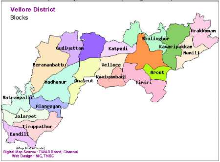
Fig 2. List of village blocks in vellore district [courtesy:]
Table 9 . Notation Representation
|
Management Measures |
Abbreviation |
Notation |
|
Crop Variety |
CV |
a 1 |
|
Growing Season |
GS |
a 2 |
|
Growth duration of the rice variety from transplanting to harvest |
GD |
a 3 |
|
Total Yield of field area |
TYF |
a 4 |
|
Managing Organic manures, straw and green manure |
OSGM |
a 5 |
|
Crop establishment Method |
CEM |
a 6 |
|
Texture of the soil |
TS |
a 7 |
|
Apply organic materials |
AOM |
a 8 |
|
Nitrogen (N) , potassium (P), phosphorous (K) supplies |
NPK |
d |
In particular, we randomly divided the 125 dataset into the training data set of 70 records (55%) and the testing data set of 55 records (58%). As we discussed in section III, Table 9 represents an information table with eight condition attributes and one decision attribute. Using the help of domain expertise we aim to derive rules from the training data to decide the amount of fertilizer usage. To discrete the information system, we need to translate values of decision and condition attributes from qualitative to quantitative form (yes,no,low,medium, high)
Table 11. Sample Training Dataset
|
Objects |
CV (a 1 ) |
GS (a 2 ) |
GD (a 3 ) |
TYF (a 4 ) |
OSGM (a 5 ) |
CEM (a 6 ) |
TS (a 7 ) |
AOM (a 8 ) |
N:P:K (d) |
|
1 |
1 |
1 |
1 |
1 |
1 |
1 |
1 |
1 |
4 |
|
2 |
1 |
1 |
1 |
1 |
2 |
1 |
1 |
1 |
4 |
|
3 |
1 |
1 |
1 |
2 |
1 |
1 |
1 |
1 |
5 |
|
4 |
1 |
1 |
1 |
2 |
2 |
1 |
1 |
1 |
5 |
|
5 |
1 |
1 |
1 |
3 |
1 |
1 |
1 |
1 |
8 |
|
6 |
1 |
1 |
1 |
3 |
2 |
1 |
1 |
1 |
8 |
|
7 |
1 |
1 |
1 |
1 |
1 |
1 |
2 |
1 |
4 |
|
8 |
1 |
1 |
1 |
1 |
2 |
1 |
2 |
1 |
4 |
|
9 |
1 |
1 |
1 |
2 |
1 |
1 |
2 |
1 |
5 |
|
10 |
1 |
1 |
1 |
2 |
2 |
1 |
2 |
1 |
5 |
|
11 |
1 |
1 |
1 |
3 |
1 |
1 |
2 |
1 |
8 |
|
12 |
1 |
1 |
1 |
3 |
2 |
1 |
2 |
1 |
8 |
|
13 |
1 |
1 |
2 |
1 |
1 |
1 |
1 |
1 |
1 |
-
A. Rule Generation
Training dataset is employed to derive minimal subset of attributes (reduct) to ensure quality of classification and final rules are selected using expert knowledge. We have also removed identical rules and odd rules to avoid complexity. For each reduct the number of supporting objects is summarized. The candidate rules are generated based on supporting count. With a criterion of minimum two supporting count initially 43 candidate rules were formed later they were minimized to 16 (table 12) with domain knowledge.
Table 12. Decision Ruleset
|
Rule |
Description |
Support |
Nonsupport |
|
|
[1] |
IF |
Crop establishment method is transplanting and total yield of field is 4-5 t/ha |
23 |
0 |
|
THEN |
Nutrition supplement N:P:K is 13:5:0 |
|||
|
[2] |
IF |
Crop establishment Method is transplanting and field is in low lying area |
15 |
0 |
|
THEN |
Nutrition supplement N:P:K is 47:10:00 |
|||
|
[3] |
IF |
Crop establishment method is transplanting ,total yield of field is 4-5t/ha and field is in low lying area |
3 |
4 |
|
THEN |
Nutrition supplement N:P:K is 66:15:10 |
|||
|
[4] |
IF |
total yield of field is 4-5t/ha and field is not in low lying area |
5 |
3 |
|
THEN |
Nutrition supplement N:P:K is 66:15:10 |
|||
|
[5] |
IF |
Crop establishment method is transplanting and total yield of field is 6-7 t/ha |
3 |
3 |
|
THEN |
Nutrition supplement N:P:K is 97:20:21 |
|||
|
[6] |
IF |
Grow duration is 100-109 days , total yield of field is 5-6 t/ha and field is in low lying area |
5 |
5 |
|
THEN |
Nutrition supplement N:P:K is 97:20:21 |
|||
|
[7] |
IF |
Grow duration is 90-99 days and growing season is dry |
4 |
9 |
|
THEN |
Nutrition supplement N:P:K is 106:25:32 |
|||
|
[8] |
IF |
Growing season is dry, Crop establishment method is transplanting and field is not in low lying area |
4 |
3 |
|
THEN |
Nutrition supplement N:P:K is 100:25:30 |
|||
|
[9] |
IF |
Growing season is wet and field is in low lying area |
2 |
5 |
|
THEN |
Nutrition supplement N:P:K is 114:30:20 |
|||
|
[10] |
IF |
Total field yield is 5-6t/ha and field is not in low lying area |
2 |
6 |
|
THEN |
Nutrition supplement N:P:K is 114:30:20 |
|||
|
[11] |
IF |
Growing season is dry and growing duration is 110-119 days |
1 |
5 |
|
THEN |
Nutrition supplement N:P:K is 114:30:20 |
|||
|
[12] |
IF |
Crop establishment method is dry seedling |
1 |
6 |
|
THEN |
Nutrition supplement N:P:K is 114:30:20 |
|||
|
Rule |
Description |
Support |
Nonsupport |
|
|
[13] |
IF |
Growing duration is 100-109 days, total field yield is 6-7 t/ha and field is in low lying area |
1 |
3 |
|
THEN |
Nutrition supplement N:P:K is 114:30:20 |
|||
|
[14] |
IF |
Growing season is wet and field is in low lying area |
3 |
6 |
|
THEN |
Nutrition supplement N:P:K is 126:35:26 |
|||
|
[15] |
IF |
Growing duration is 100-119 days, total field yield is 6-7 t/ha and field is not in low lying area |
3 |
5 |
|
THEN |
Nutrition supplement N:P:K is 126:35:26 |
|||
|
[16] |
IF |
Growing season is dry and growing duration is 100-109 days |
17 |
0 |
|
THEN |
Nutrition supplement N:P:K is 136:35:26 |
|||
|
Note* If straw is retained then P:K ratio is to be increased by 5-10 gms |
||||
Table 13.Candidate Rules
|
Rules |
CV |
GS |
GD |
TYF |
OSGM |
CEM |
TS |
FL |
NPK |
|
[1] |
x |
x |
x |
1 |
x |
1 |
x |
x |
1 |
|
[2] |
x |
x |
x |
1 |
x |
x |
x |
1 |
4 |
|
[3] |
x |
x |
x |
2 |
x |
1 |
x |
1 |
5 |
|
[4] |
x |
x |
x |
1 |
x |
x |
x |
2 |
5 |
|
[5] |
x |
x |
x |
3 |
x |
1 |
x |
x |
6 |
|
[6] |
x |
x |
3 |
2 |
x |
x |
x |
1 |
6 |
|
[7] |
x |
2 |
1 |
x |
x |
x |
x |
x |
7 |
|
[8] |
x |
2 |
x |
x |
x |
1 |
x |
2 |
7 |
|
[9] |
x |
1 |
x |
x |
x |
x |
x |
1 |
8 |
|
[10] |
x |
x |
x |
2 |
x |
x |
x |
2 |
8 |
|
[11] |
x |
2 |
2 |
x |
x |
x |
x |
x |
8 |
|
[12] |
x |
x |
x |
x |
x |
2 |
x |
x |
8 |
|
[13] |
x |
x |
3 |
3 |
x |
x |
x |
1 |
8 |
|
[14] |
x |
1 |
x |
x |
x |
x |
x |
2 |
9 |
|
[15] |
x |
x |
2 |
3 |
x |
x |
x |
2 |
9 |
|
[16] |
x |
2 |
3 |
x |
x |
x |
x |
x |
10 |
-
VII. Performance Analysis
To evaluate the performance, the proposed algorithm is validated against the real time data set of Vellore district . Two series of experiments were performed: one model on the original unreduced data and other on the reduced candidate rules. The rough based reduction algorithm selected five out of seven attributes. This reduced dataset (candidate rules) was reasonably information rich without redundant attributes. Using candidate rules (table 12) we examined the testing data set for accuracy, precision and recall measures. We observe that rules 1,2,3,4,5,6,7,8,16 are above threshold value 40%, other rules are discarded as it fails to reach threshold value. Two feature selection algorithms based on fuzzy and ANFIS versus the proposed algorithm have been applied for test and comparative measures (table 14). The results proved that our model avoids over fitting and produces sustainable results (table 15).
Table 14. Evaluation Measures
|
Category |
No of data set |
Precision |
Recall |
Accuracy (%) |
|
Rule 1 |
23 |
0.97 |
1.0 |
100 |
|
Rule 2 |
15 |
0.99 |
1.0 |
100 |
|
Rule 3 |
7 |
0.734 |
0.93 |
40 |
|
Rule 4 |
8 |
0.815 |
1.0 |
62 |
|
Rule 5 |
6 |
0.7335 |
0.75 |
50 |
|
Rule 6 |
10 |
0.75 |
0.72 |
50 |
|
Rule 7 |
13 |
0.73 |
0.723 |
42 |
|
Rule 8 |
7 |
0.834 |
0.733 |
57 |
|
Rule 9 |
7 |
0.576 |
0.51 |
28 |
|
Rule 10 |
8 |
0.671 |
0.61 |
33.33 |
|
Rule 11 |
6 |
0.376 |
0.26 |
16 |
|
Rule 12 |
7 |
0.341 |
0.29 |
16.67 |
|
Rule 13 |
4 |
0.33 |
0.31 |
16.67 |
|
Rule 14 |
9 |
0.65 |
0.68 |
33.33 |
|
Rule 15 |
8 |
0.71 |
0.59 |
33.33 |
|
Rule 16 |
17 |
0.99 |
1.00 |
100 |
Table 15. Comparative Results Of Generated Reducts
|
Algorithm |
No of Initial Attributes |
Attributes after reduction |
No of Records |
|
Rough Set |
9 |
7 |
125 |
|
Fuzzy Rough Set |
9 |
4 |
125 |
|
Unsupervised |
9 |
9 |
125 |
-
VIII. Conclusion
In Intensive cropping systems, knowledge of optimized fertilizer usage is important for developing future nutrient management strategies. This paper uses rough set theory as a useful data mining tool to depict the discovered knowledge in a direct way for nutrition management by inferring the appropriate physical conditions. This criterion is especially important in the agricultural domain because of the need for rule testability and verification by domain experts. The interesting measures such as support and confidence associated with the proposed model leads to minimized number of finalized decision rules with more accuracy. The experimental results proved to be feasible and efficient after testing with real time dataset that appropriately represents expert’s decision processes. In Future, Rough set model can be hybridized with fuzzy, genetic, entropy measures to solve multi attribute based decision making.
References Rough Set Model for Nutrition Management in Site Specific Rice Growing Areas
- Z. Pawlak, “Rough Sets: Theoretical Aspects of Reasoning about Data”, Kluwer Academic Publishers, Dordrecht, The Netherlands, 1991 .
- Dr. K.V. Rao , “Site–Specific Integrated Nutrient Management for Sustainable Rice Production and Growth”, from internet,2012,http://www.rkmp.co.in
- M. Magnani, “Technical Report on Rough Set Theory for Knowledge Discovery in Data Bases”, from internet, 2003.
- P.S. Swathi Lekshmi,K Chandrakandan and N Balasubramani, “Yield Gap Analysis among Rice Growers in North Eastern Zone of Tamil Nadu”,Agricultural Situation in India, vol. 63 no. 2,pp 729-773, 2006,
- Z.Pawlak , “Rough Sets”, International Journal of Computer and Information Sciences, vol 11, no. 5, pp 341–356, 1982.
- T. Y. Lin, Y. Y. Yao and L. A. Zadeh , “Data Mining, Rough Sets and Granular Computing”, Physica– Verlag, pp.102-124, 2002.
- Z. Pawlak and A.Skowron, “Rudiments of rough sets”, Information Sciences, Elsevier,vol.177 ,no. 1,pp 3–27, 2007.
- Qiang Shen and Alexios Chouchoulas, “Rough Set – Based Dimensionality Reduction for Supervised and Unsupervised Learning”, International Journal of Applied Mathematics and Computer Sciences, vol. 11, no. 3, pp 583-601, 2001.
- Jiye Li and Nick Cercone, “Discovering and Ranking Important Rules” ,KDM Workshop, 2006, Waterloo, Canada, Oct 30-31,pp.152-171
- S Joseph, PP Ouseph, “Assessment of nutrients using multivariate statistical techniques in estuarine systems and its management implications: a case study from Cochin Estuary, India”, Water and Environment Journal,vol 24, no. 2, pp 126-132, 2010.
- N.Xiong, and L.Litz, “ Reduction of fuzzy control rules by means of premise learning - method and case study” , Fuzzy Sets and Systems, vol.132,no.2,pp217-231.2002.
- J.Han , X.Hu and T.Y. Lin, “ Feature Subset Selection Based on RelativeDependency between Attributes” , Rough Sets and Current Trends in Computing: 4th International Conference, RSCTC Uppsala,Sweden,June1-5,pp.176–185,2004.
- A.Kangaiammal, R.Silambannan, C.Senthamarai,M.V. Srinath, “Student Learning Ability Assessment using Rough Set and Data Mining Approaches”, IJMECS vol. 5, no. 5, June 2013
- Ali Khazaee, “Heart Beat Classification Using Particle Swarm Optimization”, IJISA,vol. 5, no. 6, May 2013
- CN. Mac Parthaláin,., R.Jensen and Q.Shen, “ Fuzzy entropy-assisted fuzzy rough feature selection”, Proceedings of the 15th International Conference on FuzzySystems,pp423-430,2006
- M.G. Smith and L.Bull , “Feature construction and selection using genetic programming and a genetic algorithm”, Proceedings of the 6th European Conference on Genetic Programming , EuroGP Essex,UK,April,vol 14-16,pp229–237,2003
- X.Y. Wang, J.Yang, X.Teng , W.Xia, Wand R.Jensen,“Feature Selection based on Rough Sets and ParticleSwarmOptimization”,PatternRecognitionLetters,vol. 28,no. 4,pp 459–471, 2004,
- P. Mitra, C.A.Murthy and S.K Pal, “Unsupervised feature selection using feature similarity”, IEEE Transactions on Pattern Analysis and Machine Intelligence,Washington, DC, USA ,vol 24,pp 301-324, 2004,
- Liu , Huan and Hiroshi Motoda, “Computational methods of feature selection”. Chapman and Hall/CRC,2007.
- K.Zuhtuogullari , N.Allahverdi and N.Arikan, “Genetic algorithm and rough sets based hybrid approach for reduction of the input attributes in medical systems”,International Journal of Innovative Computing, Information and control,vol.9,no.7,pp 3015-3037,2013
- X.Pan and S. Zhang, “ Remote sensing image feature selection based on á-torrent rough set theory” , 7th International Conference on Fuzzy Systems and Knowledge Discovery, Yantai, Shandong,China,pp.1034-1038,August2010
- C.C Hsiao, , Yi-Wei Ku , “ A predictor from numerical data based on fuzzy sets and rough sets”, 3rd International Workshop on Advanced Computational Intelligence, IWACI,Suzhou, China, August 25-27 ,pp.139-144,2010.
- N.Ishii , Y.Morioka, H.Kimura,Y.Bao, “Classification by multiple reducts-KNN with confidence”, 11th International Conference on Intelligent Data Engineering and Automated Learning,Paisley,UnitedKingdom,,vol 6283,pp94-101, September1-3,2010
- N.M. Parthaláin, R.Jensen , Q.Shen, “ Finding fuzzy-rough reducts with fuzzy entropy” , IEEE international conference on fuzzy systems, Hong Kong, China, pp.1282-1288, June 1-6 2008
- A.Abraham, H.Liu, “Swarm Intelligence based rough set reduction scheme for support vector machines”, IEEE International Conference on Intelligence and Security Informatics,Taipei, Taiwan, pp. 200-202, June 17-20 2008.
