Rule Based Ensembles Using Pair Wise Neural Network Classifiers

Автор: Moslem Mohammadi Jenghara, Hossein Ebrahimpour-Komleh

Журнал: International Journal of Intelligent Systems and Applications(IJISA) @ijisa

Статья в выпуске: 4 vol.7, 2015 года.

Бесплатный доступ

In value estimation, the inexperienced people's estimation average is good approximation to true value, provided that the answer of these individual are independent. Classifier ensemble is the implementation of mentioned principle in classification tasks that are investigated in two aspects. In the first aspect, feature space is divided into several local regions and each region is assigned with a highly competent classifier and in the second, the base classifiers are applied in parallel and equally experienced in some ways to achieve a group consensus. In this paper combination of two methods are used. An important consideration in classifier combination is that much better results can be achieved if diverse classifiers, rather than similar classifiers, are combined. To achieve diversity in classifiers output, the symmetric pairwise weighted feature space is used and the outputs of trained classifiers over the weighted feature space are combined to inference final result. In this paper MLP classifiers are used as the base classifiers. The Experimental results show that the applied method is promising.

Еще

Classifier Ensemble, Pair Wise Classifiers, Rule Based Ensemble, Neural Network, Classifier Combination

Короткий адрес: https://sciup.org/15010678

IDR: 15010678

Текст научной статьи Rule Based Ensembles Using Pair Wise Neural Network Classifiers

Published Online March 2015 in MECS

Recently, to improve the performance of classification tasks, the ensemble techniques have been used. the robustness, resistance, accuracy and generality are combinational methods advantages in contrast of single classifier [1]. The ensemble procedure is based on an optimistic idea that the performance of combination of several classifiers will be improved [2]. However, the individual classifier’s accuracy and its result diversity is the base of this idea. The mentioned conditions are conflicting and requires an adequate trade-off between them.[3]. Also, Kuncheva in [4] using Condorcet Jury theorem [5], has shown that combination of classifiers can usually operate better than single classifier. The error reduction of classifiers ensemble considerably are related to the classifiers diversity. The generative and non-generative methods are two categorization of classifiers ensemble. The base classifiers diversity reinforcement is the subject of generative mode that is gained by manipulating dataset or creating different classifiers by different algorithms [6]..furthermore the concept of diversity plays an important role in the ensemble generation and could be achieved by manipulating the initial conditions of the architecture, training data, topology and training algorithm of the base classifiers [7]. Various combination methods have been proposed [8] such as classifier selection, Majority Voting, Weighted Majority Voting, Decision Templates, Naïve Bayesian fusion, fuzzy integral, behavior knowledge space , boosting , bagging and so on. Woods et al. [9] categorized the combination methods into two categories:

Dynamic classifier selection: in this category, the feature space is divided into several local regions and each region is assigned to a highly competent classifier. The principle is that, given the initial pool C, the best performing subset of classifiers in P(C) must be found, and this is the powerset of C defining the population of all possible candidate ensembles C j [10] .

Classifier fusion: in this category, the base classifiers are applied in parallel and equally experienced in some ways to achieve a group consensus [8] . classifier fusion is based on a hope that each classifier makes independent errors [10] .

The paper is organized as follow. In section 2, we review related works. In section 3, we discuss the overfitting problem in classifiers. In section 4, the proposed method for decision making from classifier output stream are discussed. In section 5 experimental results and conclusion are discussed.

II .Related Works

Rule based classifiers are used in many scope of classification tasks [11]. Usually, rules are used in the individual classifiers such as decision tree rules but recently a new ensemble method for learning compact disjunctive normal form (DNF) rules are developed[11]. The developed method produces strong results with almost linear time complexity relative to the number of rules on a wide variety of classification problems. Parvin at al. in [12] have proposed a new classification ensemble method which uses small number of diverse classifiers using manipulation of dataset structures. The classifiers efficiency and accuracy are the expressed reasons for using combination of classifiers [13]. It is observed that the same pattern misclassification in different classifiers is not simultaneously. The complementariness of base classifiers and the combination method are the success base of classifier ensemble systems[8]. Neural network ensemble is a special field of classifier ensemble. During recent years, neural network ensemble is becoming a hot spot in machine learning and data mining [14-16]. It is also considered in image processing tasks. Also neural networks can be used for making bank decision[17]. Most previous works either focused on how to fuse the outputs of multiple trained networks or how to directly design a good set of neural networks [18]. Govindarajan proposed a hybrid classification method ensemble based on Radial Basis Function (RBF) and Support Vector Machine (SVM) [19]. As mentioned, a strong ensemble is combined the individual classifiers that have not only accuracy but also diversity too. In other words, the individual classifiers errors didn’t occur on same parts of the input space[2, 20]. Some researchers to construct ensembles adopt different topologies, initial weigh setting, parameter setting and training algorithm to obtain diverse individual classifiers. For example, Rosen in [21] adjusted a training algorithm by introducing a penalty term to hearten individual networks to be decorrelated. Also, the negative correlation learning to generate negatively correlated individual neural network is proposed in [22]. Other proposed methods to create neural network ensemble, called selective approach, select the diverse individual classifiers from a pool of trained accurate networks. For example, Opitz and Shavlik in [23] have presented an algorithm called ADDEMUP which uses genetic algorithms to explicitly search for a highly diverse set of accurate trained networks. Redundant classifiers are pruned to eliminate the bias effect of them on classifier selection [24]. Another selective algorithm are proposed based on bias and variance decomposition by Navone et al. in [25]. Fu et al. in [14] were introduced a PSO based approach to select the ensemble components. In this paper, a new method to make diversity in baseline MLP classifiers is introduced. It is done by manipulating the feature set.

III. Over fitting and Diversity

Over fitting is a common phenomenon in many real world problems which aren't enough data available. Weak generalization ability due to Fitting on training data is the consequence of over fitting. The small change in training data causes different model that each model influences on the learning exercise results. In classifier ensembles high diversity is a requirement to derive benefit from the aggregating exercise[26]. So the individual classifiers created by different feature subsets should be produce strong ensembles. Compromise between diversity and accuracy is essential to create a good ensemble. Over fitting is a key problem in supervised machine learning tasks. It is the phenomenon detected when a learning algorithm fits the training set so that noise and the peculiarities of the training data are memorized. As a result of this, the learning algorithm's performance drops when it is tested in an unknown dataset. The amount of data used for the learning process is fundamental in this context [10]. Small datasets are more prone to over fitting than large data sets [27]. There are several methods to create diverse classifiers such as Random Subspace, Bagging and Boosting. The Random Subspace method creates various classifiers by using different subsets of features to train them. Bagging generates diverse classifiers by randomly selecting subsets of samples to train classifiers [28]. There are several tradition methods to improve the total accuracy of classification using diversified training set. Bagging, boosting and NNCG[1] are examples of these methods which mentioned above. The base idea of these methods is same that try to present samples to learner element according to their error rate in classifier. In fact samples are handled to have a tendency for high accuracy in classifying of test set. In ensemble classifiers, we follow output of classifiers. In proposed method, we try to handling over fitting and diversity in classifier ensembles.

IV. Proposed Method

The base idea of this paper is diversifying in base classifier’s outputs instead classifier’s inputs using complement weighted feature sets. In this paper we try to affect the final result of classifier ensemble with variance of classifiers results. pairwise classifiers are constructed to support all the samples and to use for ensembling in proposed method. The main idea is that, if a sample has been classified wrongly by some classifiers, classified truly by others which are their complements. Table 1., illustrates raw idea of proposed method in this paper. Sample 17 in table 1. has been classified wrongly by all classifiers except C2 and C5. It means that the mistake of wrong classifiers can be covered by C2 and C5 but in sample 25 there isn't any classifier to cover the mistake of classification. For this we can select some classifiers to rebuilding. In this case the robustless classifiers are potential for renovation. In our example table, C2 and C6 are appropriate.

Table 1. error matrix for some samples (all numbers are artificial)

Classifier Samples	error
Classifier Samples	1	17	25	73	95	114
C1	0.9	1	0.5	0	0.1	0.8
C2	0.7	0	0.7	0.4	0.5	0.6
C3	0	0.8	1	0	0.2	0.1
C4	0	1	0.4	0.3	0.8	0
C5	0.1	0	0.8	0.2	0	0.2
C6	0.3	0.7	0.9	0.6	0.4	0.7
C7	0.2	0.9	0.6	0	0.1	0

The flowchart of proposed method is shown in fig.1. Flowchart components will be discussed subsequently.

V. Feature manipulating method

Manipulating of original feature set by complement weighting are done to Create diversity in classifier outputs by randomly pair wise weighting original features like table 2. . We suppose that, there are four classifiers with the weighted inputs by each column in table 2. Column A In table 2., is a mask on features and in this example we assumed that there are 10 features per instance. In fact, there is only feature weighting instead feature selection. According to the number of classifiers in ensemble, masks are generated randomly and pairwisely to make diversity in original data set. Generating diversity in classifiers results is the main reason to pairwise weighting. In another word, this weighting is done to avoid same result generating in all classifiers and over fitting occurrence. The pairwise complementary weights can be in two forms, a randomly real number in range [0,1] or a binary number (0 or 1).

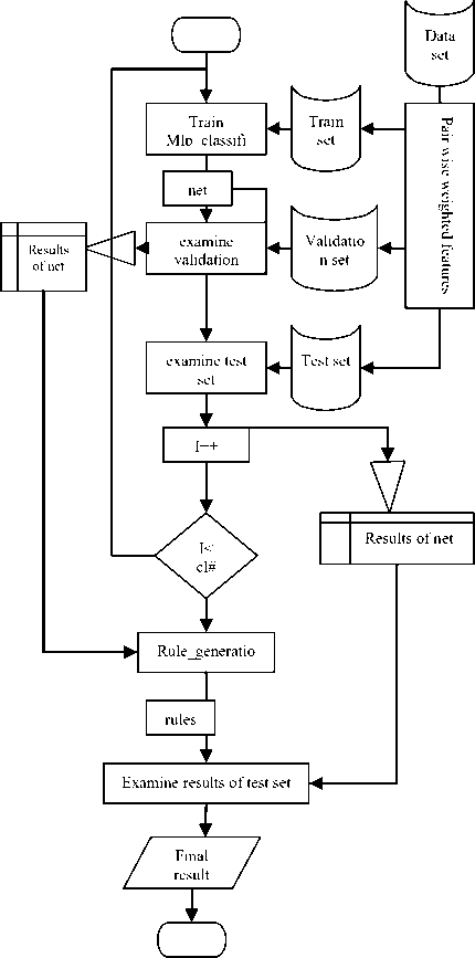
Fig. 1. flowchart of proposed method

After feature manipulating by weighting original features, samples are splitted to three disjoint subsets to use in training, validation and testing. The weight masks must be maintained to use in testing stage. As mentioned in proposed method flowchart, after feature weighting the base classifiers are trained using train set. Afterwards, the validation set samples are tested by these classifiers so results and the statistics are saved in disjoint table that we call it Rule-Pattern table . These results and their statistics are used to generate rules for applying on test set. Essentially, the generated rules functionality which is based on probability and output results diversity operate as Bays theorem. Table 3., shows an artificial example that how to use this table, will be described.

The number 27 below the AA' column in right hand of table 3., means that the result of these two classifiers on validation set is 11 over 27 samples which their actual class is 1 too. Also the number 14 in end row CC' column means that in 14 cases of samples classifier C classified as class 2 but classifier C' classified as 1, so that the true class is 1. In proposed method, these results and statistics are used to generate final result. an unknown sample for test after weighting with saved weight sets, are supplied to ensemble classifiers and the result of them are formed like table 3., that an example is showed in table 4. The generated result pattern will be searched in the RulePattern table. Assumed that two Rules which shown in table 5. are matched with the pattern shown in table 4.

The total value to decision making are computed using sum and standard deviation of matched patterns. As shown in table 5. only the majority voting or averaging don’t have efficiency, and the less standard deviation are efficient.

total value = S * — - — —

(\std + E (1)

Where S in (1) is the total sum of same patterns numbers in Rule-Pattern table. The std shows the standard deviation of result in all classifiers. The eq.1 means that the less the std the more total value. In this equation there are compromise between the sum of matched results and standard deviation. Finally the sample class is determined by total value. The class with greater total value is determined as a sample class.

VI. Experimental Results

In this paper, simple MLPs are used as the base classifiers that each one are trained with weighted train set.

Proposed method are evaluated with several Data sets that are divided into three part namely train set, validation set and test set. MLPs are trained with train set and tested with validation set. Results of this test process are saved in temporary place for rule generation phase.

To evaluate the proposed method and compare it with other related works, the Pima and the Ionosphere datasets from the UCI machine learning repository were used. Table 6. and table 7. show the result of proposed method in various parameters and conditions. All the experimental testing is performed with the same testing protocol (15 times a 10-fold cross validation) and then the average results are reported. The results were compared with averaging plain MLP and other related works.

The first row in followed tables shows the number of classifiers in ensemble. The number 8 means that there are 8 classifiers in ensemble set. The first column in tables shows the number of epoch that neural networks were trained. The number 250 means that the neural networks were trained only in 250 iterations. The other cells contain the accuracy of classifier ensemble in that situation. For example, the average ensemble accuracy with 12 classifiers and 450 epoch number is 0.6523. The accuracy is defined in (2).

Accuracy = (TP+TN) / (TP + FP + TN + FN) (2)

The experimental results on Ionosphere dataset are expressed in Table 8, table 9, table 10. and table 11. The ionosphere data set were tested in two approaches, first with randomly real number weights and second with binary weights. Table 8. and table 9. are the randomly real number weighted results and table 10. and table 11. are the binary weighting.

To compare the proposed method with related works, we use the reported result in [29] that specially works on pima data set. The comparison was showed in table 12.

The ionosphere results were compared with reported results in [30] that showed in table 13.

Table 2. pair wise feature weighting for diversifying in classifier's output ( all numbers are artificial)

A	Pair A	B	Pair B
0.655968	0.344032	0.767344	0.232656
0.508999	0.491001	0.604892	0.395108
0.299181	0.700819	0.123628	0.876372
0.851484	0.148516	0.808122	0.191878
0.510758	0.489242	0.219159	0.780841
0.842279	0.157721	0.566821	0.433179
0.756911	0.243089	0.090539	0.909461
0.047124	0.952876	0.585494	0.414506
0.139154	0.860846	0.155351	0.844649
0.409845	0.590155	0.698275	0.301725

Table 3. Rule-Pattern table.( classifiers results and statistics on validation set.( artificial))

AA'	BB'	CC'	DD'	True class	Number of each pair
AA'	BB'	CC'	DD'	True class	AA'	BB'	CC'	DD'
11	12	11	21	1	27	5	22	4
22	22	22	22	2	69	71	70	61
22	22	21	22	1	3	4	14	4

Table 4. generated results

AA'	BB'	CC'	DD'	True class
11	12	11	21	1

Table 5. matched patterns with test set pattern

c	1 , 1	2 , 2	2 , 1	1 , 2	Sum(S)	std	Total value
1	27	4	13	12	56	9.56	18.11
2	3	71	16	2	92	32.63	16.1

Table 6. experimental results on pima dataset. These results are average of several mlps

	2	4	6	8	10	12	14	16	18	20
50	0.5609	0.5844	0.6281	0.5771	0.5612	0.5824	0.6057	0.5961	0.5890	0.5843
100	0.5785	0.6324	0.6185	0.5898	0.5932	0.6098	0.5849	0.6006	0.6223	0.6112
150	0.5703	0.6227	0.6342	0.6346	0.6366	0.6133	0.6249	0.6310	0.6302	0.6405
200	0.6695	0.6602	0.6229	0.6687	0.6562	0.6732	0.6402	0.6440	0.6475	0.6412
250	0.6316	0.6357	0.6496	0.6443	0.6348	0.6169	0.6467	0.6553	0.6581	0.6554
300	0.6305	0.6377	0.6708	0.6474	0.6470	0.6708	0.6472	0.6633	0.6402	0.6577
350	0.6504	0.6568	0.6617	0.6471	0.6457	0.6357	0.6350	0.6510	0.6552	0.6500
400	0.6234	0.6750	0.6711	0.6541	0.6545	0.6174	0.6570	0.6446	0.6479	0.6519
450	0.6492	0.6477	0.6518	0.6325	0.6702	0.6523	0.6422	0.6716	0.6373	0.6509
500	0.6465	0.6564	0.6458	0.6469	0.6557	0.6544	0.6744	0.6401	0.6458	0.6479

Table 7. result of the proposed methods on pima dataset.

	2	4	6	8	10	12	14	16	18	20
50	0.7434	0.7145	0.8067	0.6434	0.7520	0.7458	0.7450	0.6536	0.7763	0.6208
100	0.7161	0.7216	0.6997	0.7575	0.7231	0.7544	0.6911	0.7169	0.7645	0.6052
150	0.6059	0.6669	0.5919	0.7075	0.7489	0.6700	0.6598	0.7755	0.7302	0.6005
200	0.6692	0.6380	0.7184	0.5966	0.7505	0.7528	0.7130	0.7231	0.7098	0.7700
250	0.7106	0.7512	0.7169	0.7919	0.7052	0.7325	0.7942	0.6848	0.8028	0.7481
300	0.7247	0.6481	0.5981	0.7216	0.6317	0.7247	0.7348	0.5958	0.7114	0.7434
350	0.5661	0.7059	0.7966	0.7278	0.7895	0.7981	0.7888	0.6989	0.7028	0.7700
400	0.6934	0.6692	0.8216	0.7700	0.5809	0.7528	0.7013	0.6513	0.8137	0.7591
450	0.6684	0.7130	0.7653	0.6739	0.6622	0.7302	0.7130	0.6669	0.7848	0.7880
500	0.7020	0.7388	0.7169	0.7091	0.7372	0.6942	0.7934	0.6708	0.7106	0.7567

Table 8. experimental result by averaging several mlps on ionosphere dataset with randomly real number weighted

	2	4	6	8	10	12	14	16	18	20
50	0.5154	0.5184	0.5587	0.5357	0.5602	0.5443	0.5490	0.5361	0.5787	0.5474
100	0.7684	0.6782	0.7120	0.7182	0.7229	0.7013	0.7034	0.7228	0.6841	0.7191
150	0.8752	0.8551	0.8470	0.8397	0.8400	0.8402	0.8425	0.8518	0.8489	0.8307
200	0.8752	0.8521	0.8709	0.8622	0.8544	0.8650	0.8503	0.8489	0.8375	0.8533
250	0.8701	0.8581	0.8587	0.8694	0.8626	0.8556	0.8501	0.8583	0.8532	0.8672
300	0.8641	0.8726	0.8510	0.8485	0.8554	0.8635	0.8498	0.8480	0.8610	0.8681
350	0.8051	0.8735	0.8499	0.8509	0.8718	0.8661	0.8529	0.8468	0.8599	0.8800
400	0.8658	0.8376	0.8564	0.8665	0.8791	0.8687	0.8604	0.8653	0.8697	0.8683
450	0.8487	0.8406	0.8818	0.8731	0.8689	0.8647	0.8847	0.8684	0.8829	0.8711
500	0.8752	0.8530	0.8453	0.8729	0.8588	0.8721	0.8717	0.8471	0.8670	0.8601

Table 9. result of the proposed methods on ionosphere dataset with randomly real number weighted

	2	4	6	8	10	12	14	16	18	20
50	0.6815	0.6969	0.5687	0.6439	0.6097	0.6610	0.5311	0.7362	0.5311	0.7038
100	0.5892	0.8764	0.8012	0.8251	0.8097	0.8200	0.8320	0.8679	0.7636	0.8644
150	0.7038	0.8918	0.8063	0.8627	0.9226	0.6781	0.9311	0.9123	0.9021	0.9209
200	0.6952	0.9448	0.9055	0.8166	0.9157	0.9414	0.9140	0.9003	0.9089	0.9174
250	0.9191	0.8422	0.8918	0.9191	0.8969	0.9123	0.8969	0.9157	0.7721	0.9311
300	0.8217	0.9191	0.9123	0.8969	0.9140	0.9174	0.9294	0.9157	0.9140	0.9277
350	0.7756	0.9397	0.9277	0.9465	0.9362	0.8320	0.9209	0.9226	0.8268	0.8935
400	0.7858	0.9198	0.8132	0.9243	0.9585	0.9021	0.9448	0.9191	0.9345	0.9277
450	0.8089	0.9352	0.7875	0.9209	0.9516	0.9055	0.8234	0.9243	0.9465	0.9243
500	0.6730	0.9226	0.9106	0.9414	0.8234	0.9294	0.9191	0.9243	0.9191	0.9482

Table 10. experimental result by averaging several mlps on ionosphere dataset with binary (0,1) weighted

	2	4	6	8	10	12	14	16	18	20
50	0.6120	0.5483	0.5695	0.5868	0.5879	0.5399	0.5712	0.5744	0.5618	0.5609
100	0.7094	0.7662	0.7279	0.7293	0.7468	0.7013	0.7234	0.7015	0.7252	0.7197
150	0.8778	0.8312	0.8370	0.8284	0.8545	0.8395	0.8385	0.8502	0.8506	0.8202
200	0.8530	0.8573	0.8456	0.8797	0.8362	0.8450	0.8705	0.8677	0.8510	0.8450
250	0.8658	0.8774	0.8613	0.8504	0.8682	0.8607	0.8408	0.8671	0.8732	0.8544
300	0.8650	0.8581	0.8783	0.8671	0.8687	0.8564	0.8557	0.8499	0.8577	0.8574
350	0.8513	0.8662	0.8658	0.8609	0.8711	0.8570	0.8667	0.8521	0.8633	0.8688
400	0.8692	0.8453	0.8516	0.8707	0.8697	0.8645	0.8652	0.8688	0.8618	0.8695
450	0.8658	0.8530	0.8718	0.8517	0.8610	0.8712	0.8703	0.8665	0.8471	0.8704
500	0.8709	0.8543	0.8419	0.8671	0.8598	0.8634	0.8668	0.8667	0.8660	0.8510

Table 11. result of the proposed methods on ionosphere dataset with binary (0,1) weighted

	2	4	6	8	10	12	14	16	18	20
50	0.7226	0.6337	0.5756	0.7072	0.5636	0.7089	0.6388	0.6867	0.6576	0.5926
100	0.6456	0.7875	0.8730	0.7756	0.8337	0.8781	0.8627	0.8679	0.8901	0.8918
150	0.8097	0.9226	0.9362	0.9209	0.9157	0.9294	0.9397	0.8200	0.9106	0.8798
200	0.8969	0.8029	0.9072	0.9448	0.9294	0.9328	0.9123	0.9328	0.9226	0.9174
250	0.8234	0.9209	0.9277	0.9191	0.8320	0.8063	0.9003	0.9379	0.9790	0.9260
300	0.8012	0.9209	0.9311	0.9397	0.9465	0.9448	0.8337	0.8969	0.9345	0.9328
350	0.9209	0.8713	0.9448	0.9362	0.9431	0.9499	0.9516	0.8439	0.8952	0.9294
400	0.9089	0.8884	0.9157	0.9328	0.9619	0.9550	0.9482	0.9465	0.9191	0.9414
450	0.9209	0.6730	0.9328	0.9397	0.9550	0.9243	0.8405	0.9533	0.9328	0.9482
500	0.9191	0.9106	0.9311	0.9431	0.7345	0.9191	0.9482	0.9397	0.9294	0.9140

Table 12. the comparison result reported on the pima data set

	KNN	Back propagation	C4.5	kohenen	Naïve bayse	Our Proposed method
pima	0.676	0.752	0.73	0.727	0.738	0.8216

Table 13. the comparison result reported on the ionosphere data set

	LDA	CTREE	CTREE Bagging	Double bagging	Proposed method with 0,1 weighting	Proposed method with real random weighting
Ionospherer	0.863	0.87	0.907	0.933	0.9619	0.9585

VII. Conclusion

We have successfully implemented and evaluated the proposed rule based ensemble classification algorithm and measured the average performance of the algorithm by considering the 10-fold cross validation. In this paper to create good ensemble, we have generated diversity in classifiers output by pair wise input feature weighting. We compared the performance of the proposed algorithm with some standard classification algorithm’s result. The Performance of ensemble classification measured with respect to accuracy. The final result shows that the proposed method accuracy is admissible in contrast to standard methods.

Список литературы Rule Based Ensembles Using Pair Wise Neural Network Classifiers

M. Mohammadi, H. Alizadeh, and B. Minaei-Bidgoli, "Neural Network Ensembles Using Clustering Ensemble and Genetic Algorithm," presented at the Third International Conference on Convergence and Hybrid Information Technology, 2008. ICCIT'08, 2008.
A. Krogh and J. Vedelsby, "Neural network ensembles, cross validation, and active learning," Advances in neural information processing systems, pp. 231-238, 1995.
H. D. Navone, P. M. Granitto, P. F. Verdes, and H. A. Ceccatto, "A learning algorithm for neural network ensembles," Inteligencia Artificial, Revista Iberoamericana de Inteligencia Artificial, vol. 12, pp. 70–74, 2001.
L. I. Kuncheva, Combining pattern classifiers: methods and algorithms: Wiley-Interscience, 2004.
L. Shapley and B. Grofman, "Optimizing group judgmental accuracy in the presence of interdependencies," Public Choice, vol. 43, pp. 329-343, 1984.
J. Kittler and F. Roli, Multiple classifier systems: Springer, 2000.
H. Zouari, L. Heutte, and Y. Lecourtier, "Controlling the diversity in classifier ensembles through a measure of agreement," Pattern Recognition, vol. 38, pp. 2195-2199, 2005.
L. Chen and M. S. Kamel, "A generalized adaptive ensemble generation and aggregation approach for multiple classifier systems," Pattern Recognition, vol. 42, pp. 629-644, 2009.
K. Woods, W. P. Kegelmeyer Jr, and K. Bowyer, "Combination of multiple classifiers using local accuracy estimates," Pattern Analysis and Machine Intelligence, IEEE Transactions on, vol. 19, pp. 405-410, 1997.
E. M. Dos Santos, R. Sabourin, and P. Maupin, "Overfitting cautious selection of classifier ensembles with genetic algorithms," Information Fusion, vol. 10, pp. 150-162, 2009.
S. Weiss, "Lightweight rule induction," ed: Google Patents, 2003.
H. Parvin, H. Alizadeh, B. Minaei-Bidgoli, and M. Analoui, "CCHR: Combination of Classifiers using Heuristic Retraining," 2008, pp. 302-305.
J. Kittler, M. Hatef, R. P. W. Duin, and J. Matas, "On combining classifiers," Pattern Analysis and Machine Intelligence, IEEE Transactions on, vol. 20, pp. 226-239, 1998.
Q. Fu, S. X. Hu, and S. Y. Zhao, "A PSO-based approach for neural network ensemble," Journal of Zhejiang University (Engineering Science), vol. 38, pp. 1596-1600, 2004.
H. Parvin, H. Alizadeh, B. Minaei-Bidgoli, and M. Analoui, "A Scalable Method for Improving the Performance of Classifiers in Multiclass Applications by Pairwise Classifiers and GA," presented at the Fourth International Conference on Networked Computing and Advanced Information Management, 2008.
Z. Wu and Y. Chen, "Genetic algorithm based selective neural network ensemble," presented at the IJCAI-01: proceedings of the Seventeenth International Joint Conference on Artificial Intelligence, Seattle, Washington, August 4-10, 2001, 2001.
M. M. Rahman, S. Ahmed, and M. H. Shuvo, "Nearest Neighbor Classifier Method for Making Loan Decision in Commercial Bank," International Journal of Intelligent Systems and Applications (IJISA), vol. 6, p. 60, 2014.
H. Parvin, H. Alizadeh, and B. Minaei-Bidgoli, "A New Approach to Improve the Vote-Based Classifier Selection," 2008, pp. 91-95.
M. Govindarajan, "A Hybrid RBF-SVM Ensemble Approach for Data Mining Applications," International Journal of Intelligent Systems and Applications (IJISA), vol. 6, p. 84, 2014.
L. K. Hansen and P. Salamon, "Neural network ensembles," presented at the IEEE Transactions on Pattern Analysis and Machine Intelligence, 1990.
B. E. Rosen, "Ensemble learning using decorrelated neural networks," Connection Science, vol. 8, pp. 373-384, 1996.
Y. Liu, X. Yao, and T. Higuchi, "Evolutionary ensembles with negative correlation learning," IEEE Transactions on Evolutionary Computation, vol. 4, pp. 380-387, 2000.
D. W. Opitz and J. W. Shavlik, "Actively searching for an effective neural network ensemble," Connection Science, vol. 8, pp. 337-354, 1996.
A. Lazarevic and Z. Obradovic, "Effective pruning of neural network classifier ensembles," presented at the International Joint Conference on Neural Networks, 2001. Proceedings. IJCNN'01, 2001.
H. D. Navone, P. F. Verdes, P. M. Granitto, and H. A. Ceccatto, "Selecting diverse members of neural network ensembles," presented at the proc. 16th Brazilian Symposium on Neural Networks, 2000.
P. Cunningham, "Overfitting and diversity in classification ensembles based on feature selection," Trinity College Dublin, Dublin (Ireland), Computer Science Technical Report: TCD-CS-2000-07, 2000.
R. Kohavi and D. Sommerfield, "Feature subset selection using the wrapper method: Overfitting and dynamic search space topology," 1995, pp. 192–197.
A. H. R. Ko, R. Sabourin, and A. S. Britto, "Pairwise fusion matrix for combining classifiers," Pattern Recognition, vol. 40, pp. 2198-2210, 2007.
Y. A. Christobel and D. P. Sivaprakasam, ""A New Classwise k Nearest Neighbor (CKNN) Method for the Classification of Diabetes Dataset" " International Journal of Engineering and Advanced Technology, 2013.
T. Hothorn and B. Lausen, "Double-bagging: Combining classifiers by bootstrap aggregation," Pattern Recognition, vol. 36, pp. 1303-1309, 2003.

Еще

Статья научная