Scaling of Digital Images by Adaptive and Combined Application of Interpolation Algorithms

Scaling of digital images is often applied in modern computer systems when processing both separate images and video stream frames [1, 2]. Scaling down of images involves reducing their dimensions (in pixels) and is used, for example, to reduce memory usage, unify a series of images to a single size, or decrease traffic of telecommunication system channels. Scaling up of images involves increasing their dimensions and is applied, for instance, to enhance visualization or restore images to their original size. Scaling of digital raster images is reduced to changing the sampling frequency for a discrete signal [3]. Changing the resolution of images is performed in various video surveillance and computer graphics systems. In scientific research, the task of image scaling arises during the processing of biomedical images [4, 5], X-ray images [6], and electron diffraction images [7]. Transformation to a specified scale is used as a preprocessing stage in computer systems for image recognition and detection [8, 9]. Since image scaling has a wide range of applications, there is currently a need to develop accurate and fast tools for changing image resolution.

Modern hardware and software tools for image scaling in most cases use interpolation algorithms that have high performance and relative simplicity of software or hardware implementation. The most common algorithms based on linear image interpolation include: nearest neighbor, Lanczos, bilinear and bicubic interpolation [3, 10]. Nonlinear image interpolation algorithms, for example, Weighted Essentially Non-Oscillatory (WENO), provide contour preservation and reduce aliasing effects [11]. In general, nonlinear image interpolation algorithms provide higher subjective quality compared to linear algorithms. However, nonlinear interpolation algorithms are characterized by higher computational complexity.

Image scaling algorithms using Fourier transform [2] and multiscale processing [12] are more complex to implement and have lower performance. A promising direction for image scaling is the use of Artificial Neural Networks (ANN), which can provide high visual quality in the resulting images. In order to minimize distortions in the scaled images, the brightness and contrast values of the images are corrected (if necessary) [13].

The possibilities of image scaling using the Pyramid Image and on Spline Model of 2-6 orders are discussed in [12]. The spline model provides smoothness for the brightness distribution of the original image, but the proposed model has a more complex software implementation compared to standard interpolation methods.

A novel image super-resolution algorithm based on bilateral quadratic interpolation is described in [14]. This algorithm is based on bilateral quadratic interpolation. According to the PSNR (Peak Signal to Noise Ratio) parameter, the proposed algorithm provides less distortion on the test set of images after interpolation than the standard bicubic interpolation algorithm. However, further research is needed to evaluate the performance of the bilateral quadratic interpolation algorithm on various types of images. Image upscaling is often performed using Convolutional Neural Networks (CNN) [2, 15], where the input consists of images at the initial scale, and the output provides images at an increased scale.

The basic architecture of the CNN for obtaining Super-Resolution images is SRCNN (Super-Resolution Convolutional Neural Network) [16]. The SRCNN architecture involves scaling the initial image to the desired size using the bicubic interpolation method, after which the pre-trained SRCNN model reduces the scaling defects in such an image. A modern method for improving image resolution using deep neural networks ESRGAN (Enhanced SuperResolution Generative Adversarial Network), which provide high quality image results, is described in [2].

The study [17] describes the modern SR3 approach, according to which Super-Resolution images are obtained through Repeated Refinement. SR3 uses denoising diffusion probabilistic models to image translation, which provides photorealistic quality of scaled images. Similar to the SRCNN architecture, the SR3 approach involves scaling the original image to the desired size using bicubic interpolation. The possibilities of obtaining Super-Resolution images by jointly using deep convolutional neural networks (CNN) and transformers are considered in the work [18]. It is shown that such a combination provides high accuracy of scaled images even in the presence of noise in the original images. In [19] a novel multi-branch residual hybrid attention block (MBRHAB) is applied to improve the image scaling accuracy. Experimental studies have shown that the MBRHAB method outperforms existing Super-Resolution algorithms (including bicubic interpolation, SRCNN, ESRGAN, Real-ESRGAN) in terms of PSNR (Peak Signal-to-Noise Ratio) and SSIM (Structural Similarity Index) metrics.

Neural network image upscaling using the Spiking Neural Network (SNN) architecture is described in [20]. Unlike traditional ANN, which work with continuous signal values, SNN use discrete pulses (spikes), similar to pulses in a biological neural network. SNN provide high accuracy in image upscaling, but their training process is more complex than that of traditional ANN.

Practical application of such ANN involves training on a large set of images containing pairs of low- and high-resolution images. However, scaling images using ANN is characterized by a relatively high probability of artifacts.

There are several programs designed for image scaling using neural networks. For example, the Waifu2x program is designed to increase the scale of images by 2 or 4 times (during a single operation) [21]. The program allows processing images iteratively, that is, the original images can be rescaled. Before scaling images, users can select a processing model (e.g., "photo"), the noise reduction level (ranging from low to highest), the scaling (zoom) factor, and the size of the rectangular tile within which the processing is performed. The advantages of the Waifu2x software include the ability to reduce the noise level [22, 23] in images during the scaling process.

The analysis of the above-described literature confirms that the development of accurate and fast image scaling tools is an urgent task. Comparison of interpolation algorithms with other image scaling algorithms shows that such algorithms have a number of advantages (simplicity of implementation, high speed, low probability of artifacts). For practical applications, it is advisable to use the common bilinear and bicubic interpolation algorithms [24], since the nearest neighbor algorithm gives too high an error, and the Lanczos algorithm has a lower speed.

Thus, the use of interpolation algorithms is appropriate in cases where simplicity of implementation and high speed are important. In addition, interpolation algorithms can be successfully combined with image scaling using ANN, since in many ANN (SRCNN [16], SR3 [17]) the image scaling to the desired size is performed by the interpolation algorithm, and the ANN then reduces the scaling defects. The problem is that image interpolation algorithms have relatively low accuracy. Image scaling errors lead, in particular, to the appearance of characteristic defects, blurred contours and loss of image detail [25, 26]. At the same time, practical image processing shows that the scaling accuracy depends not only on the interpolation algorithm, but also on the type of image (for example, an image with a large or small amount of details, an image with smooth or sharp changes in the brightness gradient). Since the scaling result depends on the spatial distribution of the image brightness (or the values of its color channels), it is proposed to evaluate the image type based on its average spatial period.

In this paper, it is proposed to increase the accuracy of image scaling by adaptive and combined use of interpolation algorithms. The peculiarity of the adaptive approach is that the interpolation algorithm is selected for each image depending on its spatial period. Combined use consists in the sequential use of different interpolation algorithms when reducing and increasing the scale of one image, which is practically used when transmitting images in a reduced scale through the channels of the telecommunication system.

2.    Theoretical Foundations of Image Scaling using Interpolation Algorithms

Digital color images are processed programmatically as arrays f RGB ( i , k , c ), where i = 0,..., M -1; k = 0,..., N -1; c = 0,..., Q_C -1; M is the image size in height (pixels), N is the image size in width (pixels), Q_C = 3 is the number of color channels (Red, Green, Blue) [1]. The pixel values of all color channels are converted to the range from 0 to 1. In the case of scaling an image in grayscale, it is processed as one color channel. Let us consider in more detail the main image interpolation algorithms: nearest neighbor, bilinear and bicubic interpolation, Lanczos [3].

The nearest neighbor algorithm is the simplest and consists in choosing the pixel value that is closest to the new pixel position after scaling.

According to the bilinear image interpolation algorithm, the new (scaled) pixel value is calculated through a linear combination of the values of the 4 closest pixels (to the new pixel position). When scaling images, bilinear interpolation is performed twice: along the height and along the width. Bilinear interpolation usually gives better results (compared to the nearest neighbor algorithm), but partially smooths the image.

According to the bicubic image interpolation algorithm, the new pixel value is calculated by cubic interpolation of the values of the 16 nearest pixels along two coordinates (height and width). Bicubic interpolation usually gives better results (compared to bilinear), but has a slower speed.

The Lanczos algorithm consists in calculating the new pixel value (after scaling) based on the values of neighboring pixels using the Lanczos window function (kernel). For interpolation of one-dimensional signals s ( x ), the Lanczos kernel is described by the sinc ( x / a ) function, where – a ≤ x ≤ a , a is the kernel size (in most cases a =3). Image scaling is performed using the two-dimensional Lanczos kernel. The Lanczos algorithm has a relatively slow speed, but allows to scale images with quite high accuracy, compared to other interpolation methods.

Adaptive application of interpolation algorithms consists in using an algorithm with minimal scaling error for processing a specific image.

The following three image scaling modes can be distinguished:

• 1.    Scaling down of all images (for example, to convert the sizes of the original images to the sizes of the input signals of the ANN).

• 2.    Scaling up all images (e.g. before rendering images to ensure high visual quality).

• 3.    Scaling down the original images, transmitting (or storing) such images and then scaling up them back (e.g. to reduce the amount of data transmitted in telecommunications systems; to preview images read in a reduced format; in the case of transmitting images via instant messengers).

In the first two modes, one interpolation algorithm is used (for scaling down or up). In the third mode, it is possible to use either one or a combined set of two algorithms (one algorithm is used for scaling down, and the other for scaling up).

Let us study interpolation algorithms in the most general third mode, since the first two modes are its components. In this case, image processing is reduced to 2 stages:

• 1.    Based on the initial color image f RGB ( M × N pixels), interpolation algorithm # 1 calculates the scaled image f RGBs ( M s × N s pixels); the scaling factor is defined as S c = M s / M (for example, S c = 0.5).

• 2.    Based on f RGBs , interpolation algorithm # 2 calculates the resulting image f RGBs 2 (with dimensions M × N pixels, i.e. the dimensions of the initial image).

If the scaled image f RGBs2 coincides with the original f RGB , then the scaling error is zero (perfect scaling). However, in practice, in most cases, there is a certain difference between the images f RGBs 2 and f RGB . Therefore, to estimate the scaling error [27, 28], the difference between f RGBs 2 and f RGB is calculated as the mean square error (MSE) and as the root mean square error (RMSE) by the formulas:

1      M - 1 N - 1 Qc - 1

MSE =            E E E [fRGB(i,k,c) — /RGBs2(i,k,c)]2 ,(1)

M • N • Q C i = 0 k = 0 c = 0

I 1 M-1 N-1 Qc -1r

RMSE =             E E  E fRGB (i,k,c) - fRGBs 2( i,k,c)]

M • N • Qc i=0 k=0

where M is the size of the f RGB image in height (pixels); N is the size of the f RGB image in width (pixels);

Q C is the number of color channels.

Based on MSE (1), PSNR (Peak Signal to Noise Ratio) values are also calculated [28]. The average spatial period T CR is determined for the grayscale image f n , which is calculated based on the initial color image f RGB ( M × N pixels). The values of the T CR period are needed to study the influence of the spatial distribution of image brightness on the scaling error RMSE (2). The T CR period is calculated based on the Fourier energy spectrum P S of the image f n . To simplify the processing of the energy spectrum P S , a square grayscale image f n with dimensions M d × N d pixels is used, where M d = N d = min ( M , N ). The Fourier spectrum F of the image f n is calculated as a result of the two-dimensional direct Discrete Fourier Transform (DFT) according to the formula [29, 30]

Md - 1

F (m, n) = E i=0

Nd - 1                 I          I m • i

E fn ⁽ i , ^k ) • exP l ^- j • ^{2 n}l —---7

k = 0             I       L M d - 1

+

n • k

N d ^{- 1}

where m is the number (index) of the spatial frequency in height (number of components of the height distribution); n is the frequency number in width; m = 0, 1, ..., M d - 1; n = 0, 1, ..., N d - 1; j is an imaginary unit.

To simplify the analysis of the spectrum, the origin of the variables m and n is shifted to the center of the frequency rectangle. As a result of such a shift of the origin of coordinates, the centered matrix F C is calculated based on the matrix of Fourier spectrum coefficients F [1, 31]. The Power Spectrum (or “Power spectral density”) P S is calculated as the square of the modulus of the centered spectrum F C using the equation

Ps = F C I².

Based on the energy spectrum P S , its averaged radial profile P R ( d ) is calculated, where d = 0, 1, ..., N R -1, where N R = [ M d /2] + 1. The radial profile P R ( d ) describes the dependence of the amplitudes of radial spatial frequencies (averaged for all directions) on the frequency numbers d [32]. For the energy spectrum P S the coordinates of its center M C = [ M d /2] (in height), N C = [ N d /2] (in width) are determined.

The value of PR(d) is calculated as the arithmetic mean of the energy spectrum coefficients PS(m, n), for which d = -J(m - Mc)2 + (n - Nc)2 . For each number d of radial spatial frequency its value vr is calculated vr

d

.

2( Nr - 1)

The values of spatial frequencies v r are in the range from 0 to 0.5 (pixels^-1). The average spatial frequency v CR of the image f n is calculated based on the radial profile P R ( d ) using the equation [33]:

d max              / ^d = ^d max

VCR = E Vr (d) • Pr (d)     E   Pr (d), d=d min           / d=d min where vr(d) is the spatial frequency value (5) corresponding to the number d; dmin is the minimum spatial frequency number being analyzed (e.g., dmin = 1); dmax is the maximum spatial frequency number being analyzed (e.g., dmax = NR).

The values of d min are chosen to be no less than 1, since d min = 0 corresponds to the constant component of the signal. The average spatial period T CR of the image is calculated as:

.

T CR =---- v CR

The scaling errors RMSE are calculated separately for each set of two algorithms that are used for successive image scaling down and up. To compare the accuracy of the algorithms, the relative scaling error RMSE_R is also used, which is calculated as:

RMSE

RMSE _ II RMSE I ,

where RMSE_I is the scaling error by the algorithms set I; RMSE_II is the scaling error by the algorithms set II.

The dependence of the relative scaling error RMSE_R on the values of the period T CR is mathematically described by a regression equation in the form of a polynomial of degree P d :

Pd

RMSE _ RA = b о + X b p • ( T_Cr ) ^p , p = 1

where b 0 , b 1 ,..., b Pd are the coefficients of the polynomial.

Thus, using equation (9), it is possible to investigate the influence of the spatial period T CR of images on the accuracy of their scaling.

This allows, by scaling a series of Q Im test images f RGB , to determine the threshold value T h for the spatial period T CR at which both sets of interpolation algorithms provide the same error; therefore, at T CR <  T h , one of the algorithm sets provides a smaller error, and at T CR ≥ T h , the other set provides a smaller error. The scaling error RMSE is calculated from the difference of the f RGB and f RGBs 2 images according to formula (2). After that, a regression analysis of the dependence of the relative scaling error RMSE_R (8) on the spatial period T CR for all Q Im of the studied images is performed. The regression equation is constructed in the form of a polynomial of degree P d according to formula (9), the regression coefficients are calculated by minimizing the root mean square difference RMSEb between the values RMSE_R and the corresponding values of the polynomial RMSE_RA . The threshold value of the spatial period T h is calculated as the T CR value at which RMSE_RA = 1.

3.    Software Implementation of Image Scaling

The software for scaling images by adaptive and combined application of interpolation algorithms was developed in Python [34] based on the mathematical model (1-9). The initial (input) data for the program are digital images f RGB (size M × N pixels). The initial images are read from graphic files or from a video camera. The color f RGB images are converted to grayscale and recorded in the image f n (size M d × N d pixels). For each image f n , the Fourier spectrum F , the energy spectrum P S , its averaged radial profile P R and the spatial period T CR are calculated. The direct Discrete Fast Fourier Transform (DFFT) of the image f n is performed by the fft2() function of the SciPy library.

Adaptive application of interpolation algorithms consists in the fact that the choice of algorithms is performed depending on the value of the spatial period T CR of the image. When T CR <  T h , scaling is performed by one of the algorithm complexes, and when T CR ≥ T h , by another algorithm complex (which provides a smaller scaling error). For example, if bicubic interpolation in the algorithm complex I is used to downscale and upscale of images, and bilinear interpolation in the algorithm complex II is used to downscale and upscale, then the program operation is described by the following activity diagram (Fig. 1). In this case, when T CR <  T h , scaling is performed by bilinear interpolation, and when T CR ≥ T h , by bicubic interpolation.

The scale of the initial f RGB image is downscale by S c times, i.e. the f RGB image (with size M × N pixels) is scaled to the f RGBs image (with size M s × N s pixels), where M s = S c ∙ M . Next, the image is upscale by S c times, i.e. the f RGBs is scaled to the f RGBs 2 image (with size M × N pixels). Scaling of images is performed by the resize() function of the OpenCV library using interpolation methods:

• •    INTER_LINEAR is a method that implements the bilinear interpolation algorithm;

• •    INTER_CUBIC is a method that implements the bicubic interpolation algorithm.

4.    Results and Discussion

The output data (results) of the program are scaled fRGBs2 images.

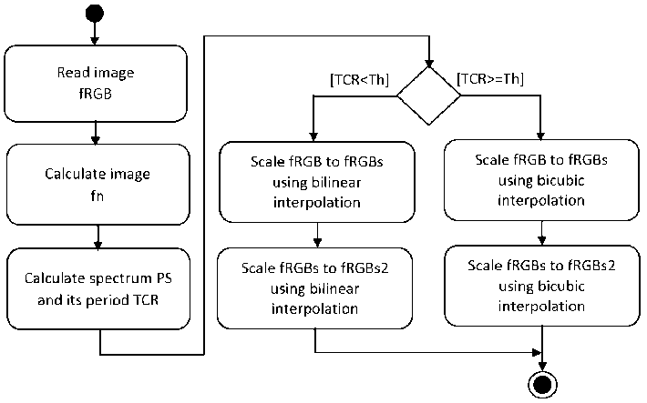
Fig. 1. Activity diagram of a software for scaling images using interpolation algorithms.

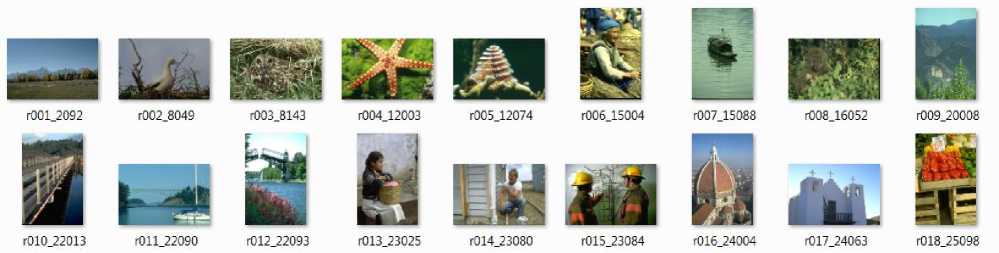
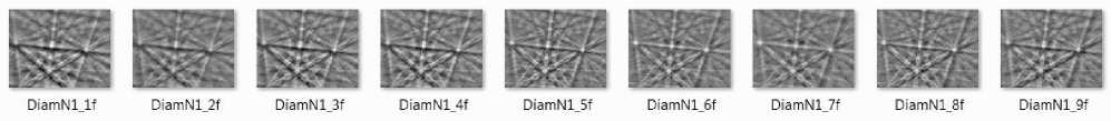
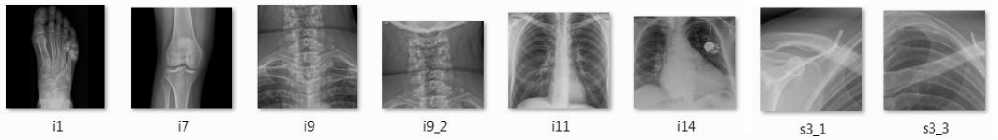
Using the developed program, the following types (subsets) of images were scaled: BSDS300 database images (Fig. 2a), Kikuchi Patterns (Fig. 2b), X-ray biomedical images (Fig. 2c), and text document images (Fig. 2d). In total, the sample contained Q Im =278 images.

(a)

(c)

tl_s300            t2_s300            t3_s3OO            t4_s300            t5_s3OO            t6_s300            t7_s300            t8_s300

(d)

Fig. 2. A fragment of dataset with QIm=278 studied images: a) BSDS300 database images (18 images from 200) [35, 36]; b) Kikuchi Patterns (9 images from 44) [7]; c) X-ray biomedical images (8 images from 17) [37]; d) text document images (8 images from 17) [22].

First, the images were scaled using a set of algorithms I (scale down and up using the bicubic interpolation algorithm) and a set of algorithms II (scale down and up using the bilinear interpolation algorithm).

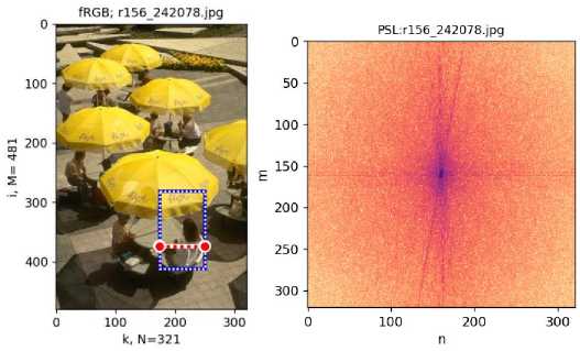
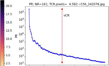
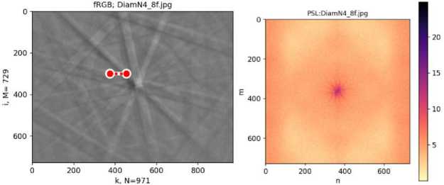
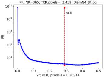
Let us consider the process of scaling image # 156 from the BSDS300 database [35, 36] (Fig. 3a). From the initial f RGB image, a square image f n in grayscale is obtained, for which the energy spectrum P S (Fig. 3b) and the averaged radial profile P R of the spectrum (Fig. 3c) are calculated. Based on the initial f RGB image, the image f RGBs (Fig. 4a) is calculated in a reduced scale (scale down by 2 times) using bilinear or bicubic interpolation algorithms. By scaling the f RGBs image using bilinear or bicubic interpolation algorithms, the image f RGBs2 is calculated in an enlarged scale (Fig. 4b, Fig. 4c, Fig. 4d). In this case, the bicubic interpolation algorithm provides a smaller scaling error RMSE (Fig. 4b) than the bilinear interpolation algorithm (Fig. 4c).

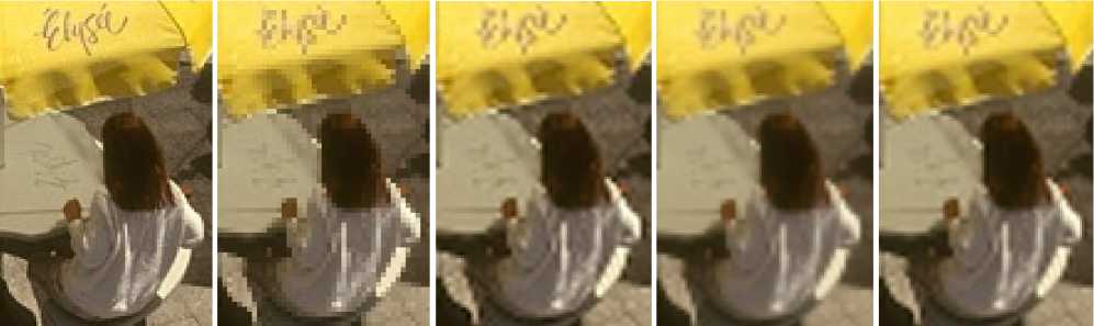
The difference between scaled images calculated by different interpolation algorithms is most noticeable in individual fragments of such images (Fig. 5) and on their profiles (Fig. 6). Certain oscillations (ringing artifacts) appear on images scaled by the bicubic interpolation algorithm (Fig. 5c, Fig. 6a). Scaling by the bilinear interpolation algorithm leads to significant image smoothing (Fig. 5d, Fig. 6b). Sequential scaling by the bilinear and bicubic interpolation algorithm (in the case of this image) provides less image distortion due to less blurring (compared to bilinear interpolation) and less oscillations (compared to bicubic interpolation) (Fig. 5e, Fig. 6c).

(a)

(b)

Fig. 3. Initial fRGB image #156 from dataset BSDS300 [34, 35] (a), its energy spectrum PS in logarithmic scale (b) and the averaged radial profile PR of the spectrum (c).

0.0       0.1       0.2       0.3       0.4       0.5

vr; vCR, pixels ! = 0.21822 (c)

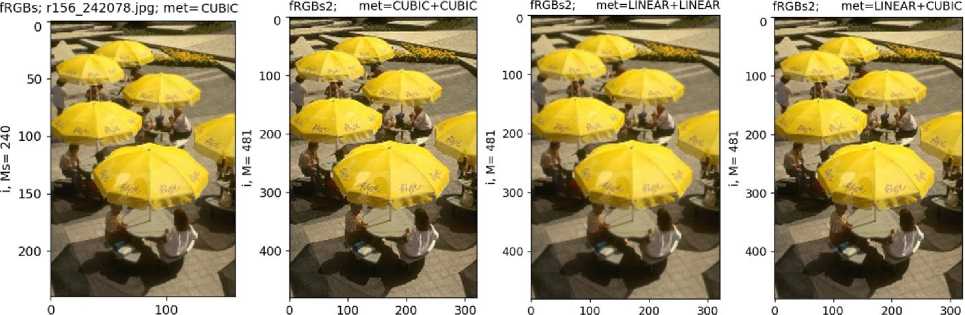
k, №=160                  k, N=321; RMSE=0.04652            k, N=321; RMSE=0.04774             k, N=321; RMSE=0.04510

(a)                                      (b)                                     (c)                                     (d)

Fig. 4. The fRGBs image in a reduced scale (a) and the fRGBs2 image in an enlarged scale, calculated by the algorithms: (b) bicubic interpolation (algorithm set I, "CUBIC+CUBIC" methods); (c) bilinear interpolation (algorithm set I, "LINEAR+ LINEAR" methods); (d) bilinear and bicubic interpolation ("LINEAR+CUBIC" methods).

For the images of the studied set (Fig. 2), the relative scaling errors RMSE_R (8) and the values for their average spatial period T CR (7) were calculated, as a result of which the dependence RMSE_R ( T CR ) was obtained (Fig. 7). The obtained dependence RMSE_R ( T CR ) is described by the regression equation RMSE_RA ( T CR ) (9), namely a polynomial of degree 2. The spatial period threshold value T h is calculated as the T CR value at which RMSE_RA = 1, so T h = 4.45 pixels (Fig. 7).

(a)                               (b)                              (c)                              (d)                              (e)

Fig. 5. Image fragments: (a) fRGB (Fig. 3a, fragment highlighted by a rectangle); (b) fRGBs in a reduced scale (Fig. 4a); (c) fRGBs2 in an enlarged scale, “CUBIC+CUBIC” methods (Fig. 4b); (d) fRGBs2 in an enlarged scale, “LINEAR+ LINEAR” methods (Fig. 4c); (e) fRGBs2 in an enlarged scale, “LINEAR+CUBIC” methods (Fig. 4d).

(a)

(b)

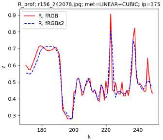
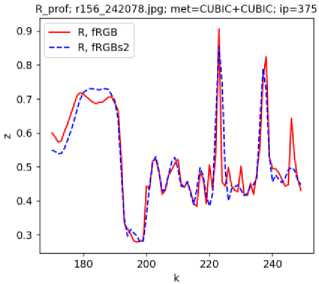
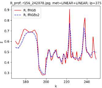
(c)

Fig. 6. Horizontal profiles of the red color channel of the initial fRGB images (Fig. 3a, the ends of the horizontal segment correspond to the beginning and end of the profile) and scaled fRGBs2 images (Fig. 4b, Fig. 4c, Fig. 4d), which are calculated by: (a) bicubic interpolation algorithms (algorithm set I, "CUBIC+CUBIC" methods, RMSE = 0.04652); (b) bilinear interpolation (algorithms set II, "LINEAR+ LINEAR" methods, RMSE = 0.04774); (c) bilinear and bicubic interpolation ("LINEAR+CUBIC" methods, RMSE = 0.4510).

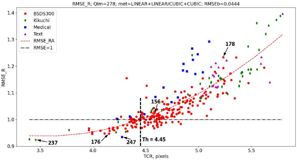
Fig. 7. Dependence of the relative scaling error RMSE_R (8) from the average spatial period TCR (7) for images of the studied dataset (Fig. 2); BSDS300 – images of the BSDS300 database, Kikuchi – images of Kikuchi Patterns, Medical – X-ray biomedical images, Text – images of text documents; RMSE_RA – regression equation (9) (polynomial coefficients b0= 1.876813, b1=-0.530587, b2=0.07490); scaled images were calculated by bicubic interpolation algorithms (algorithms set I, “CUBIC+CUBIC” methods) and bilinear interpolation (algorithms set I, “LINEAR+ LINEAR” methods); numbers 156, 176, 178, 237 and 247 correspond to images in the coordinate space RMSE_R(TCR).

The average spatial frequency of the image v CR (6) and the average spatial period T CR (7) were calculated for the minimum spatial frequency number d min = [ N R ∙ 0.25] and the maximum spatial frequency number d max = N R . Such values of the parameters d min and d max were chosen under the condition of minimizing the root mean square difference RMSEb (Fig. 6) between the values of RMSE_R and the corresponding values of the polynomial RMSE_RA (9).

The results of image scaling by bicubic and bilinear interpolation algorithms show that there is a dependence of the relative scaling error RMSE_R from the average spatial period T CR . This dependence is confirmed by the Pearson correlation coefficient Corr = 0.843428. Thus, for some images with low T CR <  T h values, the bilinear interpolation algorithm provides a smaller scaling error RMSE than the bicubic interpolation algorithm. This scaling feature is observed, for example, for the Kikuchi Patterns # 237 (Fig. 8, Fig. 9) and the X-ray biomedical image # 247 (Fig. 10, Fig. 11).

That is, the image interpolation algorithm can be chosen adaptively according to the criterion of minimizing the scaling error RMSE . The proposed method allows to reduce the scaling error, since according to the value of the spatial period T CR , images are divided into two classes: for class # 1 ( T CR ≥ T h ), the bicubic interpolation algorithm provides a smaller RMSE scaling error, and for class # 2 ( T CR <  T h ), the bilinear interpolation algorithm provides a smaller RMSE error (Fig. 7). It is advisable to perform a practical determination of the best algorithm (by the minimum RMSE ) not through the value of the T CR period (which requires a lot of computing resources), but by comparing rectangular fragments of small size (for example, 64 × 64 pixels) for the original f RGB and scaled f RGBs2 images.

(a)

(b)

(c)

Fig. 8. Initial image fRGB of Kikuchi Patterns # 237 [7] (a), its energy spectrum PS in logarithmic scale (b) and the averaged radial profile PR of the spectrum (c).

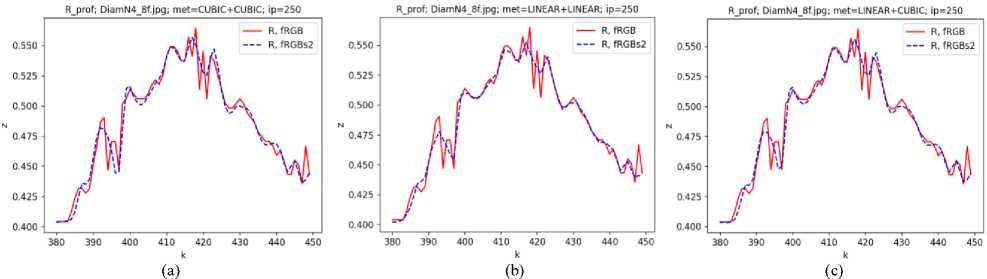
Fig. 9. Horizontal profiles of the red color channel for the fRGB image (Fig. 8a, the ends of the horizontal segment correspond to the beginning and end of the profile) and scaled fRGBs2 images, which are calculated by the algorithms: (a) bicubic interpolation (algorithms set I, "CUBIC+CUBIC " methods, RMSE=0.01637); (b) bilinear interpolation (algorithms set II, "LINEAR+ LINEAR" methods, RMSE=0.01511); (c) bilinear and bicubic interpolation ("LINEAR+CUBIC" methods, RMSE=0.01538).

(a)                                            (b)                                                            (c)

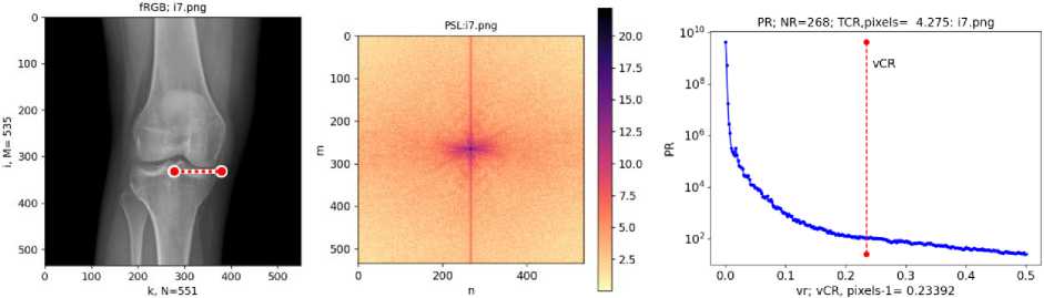
Fig. 10. Initial X-ray biomedical image fRGB # 247 [37] (a), its energy spectrum PS in logarithmic scale (b) and the averaged radial profile PR (c).

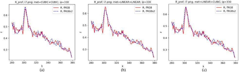
Fig. 11. Horizontal profiles of the red color channel for fRGB images (Fig. 10a) and scaled fRGBs2 images, which are calculated by the algorithms: (a) bicubic interpolation (algorithms set I, "CUBIC+CUBIC" methods, RMSE=0.01147); (b) bilinear interpolation (algorithms set II, "LINEAR+ LINEAR" methods, RMSE=0.01072); (c) bilinear and bicubic interpolation ("LINEAR+CUBIC" methods, RMSE=0.01094.

When scaling one image, it is possible to combine different interpolation algorithms. To test the capabilities of this scaling method, images were processed using an algorithm set I (scale down and up using the bicubic interpolation algorithm) and an algorithm set II (scale down using the bilinear interpolation algorithm and scale up using the bicubic interpolation algorithm). As a result of scaling the studied images (Fig. 2), their relative scaling errors RMSE_R (8) and average spatial period T CR (7) were calculated (Fig. 12).

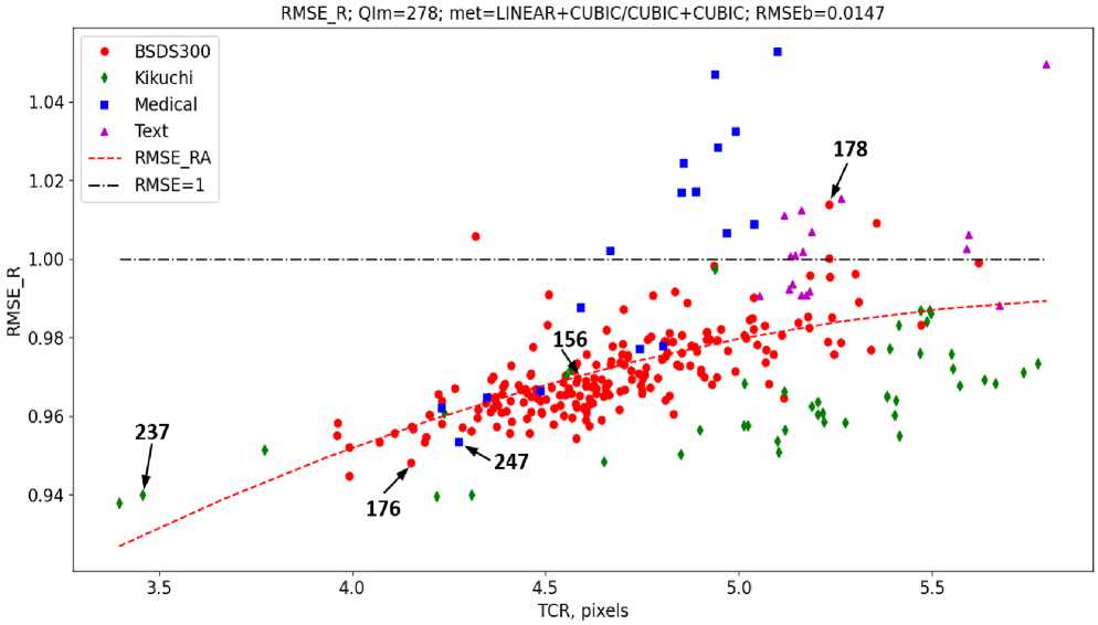
Fig. 12. Dependence of the relative scaling error RMSE_R (8) from the average spatial period TCR (7) of the images of the studied set (Fig. 2); BSDS300 – images of the BSDS300 database, Kikuchi – images of Kikuchi Patterns, Medical – X-ray biomedical images, Text – images of text documents; RMSE_RA – regression equation (9) (polynomial coefficients b0=0.667929, b1=0.105665, b2=-0.008663); scaled images were calculated by bicubic interpolation algorithms (algorithms set I, “CUBIC+CUBIC” methods), bilinear and bicubic interpolation (algorithms set II, “LINEAR+ CUBIC” methods); numbers 156, 176, 178, 237, 247 correspond to images in the coordinate space RMSE_R(TCR).

The results of image scaling (Fig. 12) show that there is a correlation between relative scaling error RMSE_R and average spatial period T CR (correlation coefficient Corr = 0.523043). For most of the studied images, the combined sequential application of the bilinear and bicubic interpolation algorithms (LINEAR+CUBIC) provides a smaller scaling error than the separate application of the bilinear (LINEAR+LINEAR) and bicubic (CUBIC+CUBIC) interpolation algorithms (Table 1).

For example, when scaling image # 156 (Fig. 3, Fig. 4), the smallest RMSE error was obtained in the case of sequential application of bilinear and bicubic interpolation algorithms ("LINEAR + CUBIC" methods), which is especially noticeable on the profiles of scaled images (Fig. 6c).

For some images, the smallest RMSE error is provided by the bilinear interpolation algorithm, for example, for the Kikuchi Patterns # 237 (Fig. 8, Fig. 9) and for the X-ray biomedical image # 247 (Fig. 10, Fig. 11). This result can be explained by the presence of a significant level of noise in the images (Fig. 8a, Fig. 10a), since the use of bilinear interpolation leads to smoothing and reduction of the noise component in the image after scaling.

The scaling of the studied images was also performed by the Lanczos algorithm (LANCZOS+LANCZOS) and by combining bilinear interpolation with the Lanczos algorithm (LINEAR+LANCZOS) (Table 1). However, when processing images by reducing and increasing the scale, the Lanczos algorithm provides a greater error (compared to the combination of bilinear and bicubic interpolation), and at the same time has a lower speed. Therefore, for such image scaling, it is more expedient to sequentially use bilinear and bicubic interpolation.

The hypothesis of a normal distribution of RMSE values when scaling images of the studied dataset was confirmed by the Pearson χ² criterion [38]. Based on the scaling results for each set of interpolation algorithms, the average scaling error A R and the standard deviation σ R for RMSE were calculated, and the limits of the confidence interval A Rmin <  A R <  A Rmax with a reliability of γ = 0.95 were also calculated [38] (Table 1, Fig. 13).

Table 1. Average scaling error A R and standard deviation σ R for RMSE values, confidence interval limits A Rmin <  A R <  A Rmax for a dataset of Q Im = 278 images (Fig. 2).

	CUBIC+CUBIC	LINEAR+LINEAR	LINEAR+CUBIC	LANCZOS+LANCZOS	LINEAR+LANCZOS
A R	0.03624219	0.03787999	0.03530453	0.03848144	0.03555926
σ R	0.02402492	0.0255262	0.02351924	0.02548071	0.02363227
A Rmin	0.03341799	0.03487931	0.03253977	0.03548752	0.03278256
A Rmax	0.03906639	0.04088067	0.03806929	0.04147654	0.03833612

CUBIC+CUBIC

LINEAR+LINEAR

LINEAR+CUBIC

Methods

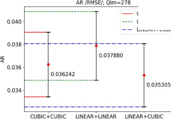
Fig. 13. Average scaling errors A R and their confidence interval limits for a series of Q Im = 278 images (Fig. 2).

Thus, according to the average scaling error A R and taking into account the limits of its confidence interval A Rmin , A Rmax , the smallest scaling error is provided by the set of bilinear and bicubic interpolation algorithms (LINEAR+CUBIC), the average value is obtained for the bicubic interpolation algorithm (CUBIC+CUBIC), and the highest error is given by the bilinear interpolation algorithm (LINEAR+LINEAR). This result confirms the effectiveness of the combined application of interpolation algorithms. However, the obtained regularities for scaling errors were obtained sequentially when reducing the image scale by 2 times and then increasing the scale by 2 times. If the image scale is first increased, then a smaller error is obtained in most cases when using the bicubic interpolation algorithm. A series of 278 images was also processed with scaling factor 3 (reduction and increase). As in the case of scaling factor 2, the smallest scaling error was obtained with the sequential application of bilinear and bicubic interpolation algorithms.

5.    Conclusion and Future Research Directions

The possibilities of increasing the accuracy of scaling digital images using bilinear and bicubic interpolation algorithms were investigated. Scaling errors were estimated through the root mean square error ( RMSE ) between the brightness of pixels of the original and scaled images. Scaling of images using interpolation algorithms and analysis of the obtained results were implemented programmatically in Python. Scaling of a dataset of Q Im = 278 images of different types was performed: images of the BSDS300 database and Kikuchi Patterns, X-ray biomedical images and images of text documents. Image processing consisted of scaling images using a set of two interpolation algorithms, namely, scale down by 2 times using algorithm # 1 and subsequently scale up by 2 times using algorithm # 2. Such processing is appropriate, in particular, for reducing the volume of data transmitted in telecommunication systems.

The influence of the average spatial period T CR of the image on the relative scaling error RMSE_R , which is equal to the ratio of the RMSE error for different interpolation algorithms, is analyzed. The period T CR is calculated based on the radial profile P R for the energy spectrum P S of the image. It is established that the dependence of the relative scaling error RMSE_R from the values of the spatial period T CR of the images is described by a regression equation in the form of a polynomial of degree 2.

A significant correlation was obtained between the values of the relative scaling error RMSE_R and the spatial period T CR of images scaled by the bicubic and bilinear interpolation algorithms. In most cases, the bicubic interpolation provides a smaller scaling error RMSE , but for some images with small values of the period T CR , the bilinear interpolation provides a smaller RMSE error. Therefore, it is proposed to increase the scaling accuracy by adaptively selecting the interpolation algorithm for each image according to the criterion of minimizing the scaling error.

The feasibility of combined use of interpolation algorithms are shown, which consists in successive scaling of one image by different interpolation algorithms. A statistical analysis of the scaling results is carried out, the average scaling error A R and the standard deviation σ R for RMSE values are calculated, and the limits of the confidence interval A Rmin <  A R <  A Rmax with reliability γ are also calculated. According to the results of statistical analysis, it is established that scaling down by the bilinear interpolation algorithm and scaling up by the bicubic interpolation algorithm in most cases provides a smaller error than the separate use of the bicubic and bilinear interpolation algorithms.

In future studies, for the highest quality image scaling, it is planned to use more complex interpolation algorithms and artificial neural networks, in particular, CNN. The proposed interpolation method can be used to calculate input images of the desired size for the SRCNN [16] and SR3 [17] methods (in which images are scaled to the desired size by the bicubic interpolation), which will allow images with fewer defects to be fed to the inputs of neural networks and ensure higher accuracy of the resulting images. The proposed method can also be implemented in telecommunication systems for transmitting images at a reduced scale and for restoring the original sizes of images.

Author Contributions Statement

Serhiy Balovsyak – Methodology, and Supervision: Proposed research ideas, Development of a mathematical model, Constructed the overall framework, and supervised project execution.

Mariana Borcha – Data Curation: Handled data acquisition, dataset preprocessing; Contributed to the literature survey.

Yurii Hnatiuk – Conceptualization: Proposed research ideas, Development of a mathematical model; Software Implementation and Statistical Analysis; Writing – Drafted the initial manuscript, contributed to the literature survey, and documented the technical background of the study.

Khrystyna Odaiska – Formal Analysis, Visualization: Performed in-depth analysis of experimental results.

Ihor Fodchuk – Writing – Review and Editing, and Project Management: Reviewed and edited the manuscript, ensured clarity and coherence, and helped coordinate project milestones and deadlines.

All authors have read and agreed to the published version of the manuscript.

Conflict of Interest

The authors declare no conflict of interest.

Funding Declaration

This research was not supported by a grant.

Data Availability Statement

This study analyzed publicly available datasets. The datasets can be found here: The Berkeley Segmentation Dataset and Benchmark. BSDS300, URL: (Last accessed: 21.02.2025)

Ethical Declarations

Statements of ethical approval for studies involving human subjects and/or animals.

Acknowledgment

We would like to express our gratitude to the reviewers for their precise and succinct recommendations that improved the presentation of the results obtained.

Declaration of Generative AI in Scholarly Writing

AI and AI-assisted technologies were not used during the writing process.

Abbreviations

The following abbreviations are used in this manuscript:

ANN - Artificial Neural Networks

CNN - Convolutional Neural Networks

DFFT - Discrete Fast Fourier Transform

DFT - Discrete Fourier Transform

ESRGAN - Enhanced Super-Resolution Generative Adversarial Network

MBRHAB - Multi-Branch Residual Hybrid Attention Block

MSE - Mean Square Error

PSNR - Peak Signal to Noise Ratio

RMSE - Root Mean Square Error

SNN - Spiking Neural Network

SRCNN - Super-Resolution Convolutional Neural Network

SSIM - Structural Similarity Index