Scheduling freight trains in rail-rail transshipment yards with train arrangements

Published Online October 2017 in MECS

Intermodal transportation [1] as well as train routing and scheduling [2] are important areas of operations’ research nowadays. Particularly, a problem of Container Processing in Railway Yards has got lots of attention recently. A survey [3] describes the problem setting and its various extensions pretty well.

One of the main issues of the Container Processing in Railway Yards area is a problem of scheduling freight trains in rail-rail transshipment yards (TYSP) [4]. The original paper [4] describes five levels of depth for the overall train scheduling problem:

• (i)    to bundle each train to a service slot, i.e. to schedule trains;

• (ii)    to assign each train of a bundle to a railway track;

• (iii)    to make a decision on positions of trains’ containers;

• (iv)    to assign container moves to portal cranes;

• (v)    to determine a sequence of moving containers for every gantry crane [4] (Fig.1).

The article [4] solves the level (i) of the problem (scheduling the service slots for trains). The article provides a mathematical model and two solution algorithms: an exact algorithm that uses dynamic programming and a heuristic algorithm that utilizes a beam search procedure. A complexity proof for given algorithms is also described there.

Later works bring further improvements to the initial mathematical model and improve solution algorithms. In [5], the original TYSP is extended by new real-world restrictions and a lot of new solution algorithms are given. In [6-9], a branch-and-bound algorithm (developed for the first time in [5]) is improved with a more effective Lagrangian lower bound.

However, [4] and all later works solve only the level (i) of TYSP (scheduling the service slots for trains).

In this article, a deeper problem of assigning every train to a railway track is considered. A mathematical model and a solving method for this problem are given here.

A distinctive feature of the given mathematical model is that Boolean variables are not used and the model mostly works with combinatorial objects (tuples of permutations). The proposed solution method is based on generation of combinatorial sets.

A problem of assigning trains to railway tracks in every service slot is considered. It could be an important task because a total cost of loading/unloading operations in real systems can depend on a distance between a source train and a target train. If a target train and a source one are served within the same time slot, it seems appropriate to place them on the closest railway tracks. If trains are served in different time slots, it is also important to place both trains in such a way that movements of the gantry crane are made as short as possible. In this case, the crane should firstly move containers from the source train to a storage area and then from a storage area to the target train. Thus, both trains should be as close to the storage area as possible.

The remainder of this paper is organized as follows.

Section 2 describes a mathematical model of the proposed approach. Section 3 gives details to a solution algorithm. Section 4 presents computational results. Conclusions are given in the final section.

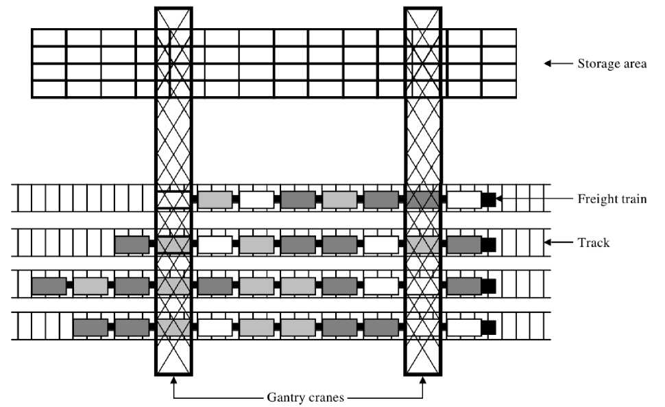
Fig.1. Representation of transshipment yard

• II.    The Mathematical Model

A mathematical model is a further extension of the one proposed in [4] as it describes a more detailed problem: the problem of assigning every train to a railway track (the level 2 according to [4]). Our model describes the problem using combinatorial structures instead of Boolean variables.

We should dwell on the problem [4] once again. There are G tracks and a given set I of trains, where each train has a predefined number of wagons and a certain load factor, defining a number of containers carried by this train. Each train is then assigned to a service slot t = 1,…, T of G simultaneously served trains. This assignment is restricted to the earliest available slot e_i of a train i (the earliest arrival time) and the latest available slot l i (the latest departure time). The transshipment yard typically deals with distinct bundles of trains (also known as service slots ). It means that G trains (one per a track) are simultaneously served and jointly leave the system after all container moves required for that bundle of trains have been accomplished. Then another bundle of G trains enters the yard [4]. Every iteration is a service slot.

Thus, some special situations are also considered in [4]:

• (1)    revisits, i.e. situations, when a train to have already

been unloaded has to enter the transshipment yard again to be loaded with items to have been delivered after the first train’s visit;

• (2)    split moves when a train i that carries a container dedicated to a train j and is served in a service slot t before a service slot t’ of the train j .

A core decision of the transshipment yard scheduling problem (TYSP) involves assigning every train i of the given train set I to a service slot t = 1,..., T [4]. In addition to [4], this article solves the problem of assigning every train to one of the tracks at each slot . At most G trains can be assigned to each slot t because G is a number of parallel railway tracks of the transshipment yard [4]. Let us construct the mathematical model of the problem in terms of combinatorial optimization.

Let’s describe each time slot t using a tuple K^t containing an amount of all trains assigned to the slot t ; we consider assigning every train to a certain railway track,     their     order     is     important,      so

K = (kt,k2,...,kg,...,kfG) . Here  kg e I denotes an amount of trains assigned to the time slot t and located on a railway track g e G.

It’s worth noting that while forming a time slot, we are choosing G trains from I possible ones, so that we are choosing  Kt  from a set of permutations  PG

(permutations of I elements are taken from G at one time). So, choosing an optimal time slot K^t can be treated as the combinatorial optimization problem of choosing the optimal permutation from the set K e p G .

In this way, decision variables are time slots

K * , * = 1,2,..., T to have been formed by the trains.

A decision result should meet three points:

• 1.    A number of trains’ revisits.

• 2.    A cost of split moves for containers (which depends on assignment of trains to railway tracks) is to be minimized.

• 3.    A cost of moves for containers between trains at the same time slot (which also depends on assignment of trains to railway tracks) is to be minimized.

The objective #1 is the same one as in [4]; the objective #2 is a more general case for the one described in [4] where an only number of split moves is considered; the objective #3 is a new one compared to [4] because trains’ assignment to railway tracks is taken into account.

As described in [4], we have the multi-objective optimization problem (the objectives #1 and #2 exist here, but the objective #3 is new) and use linear scalarization to formulate the problem as the single-objective optimization one. Let’s describe an objective function and constraints.

T T GG aZyt+«2Z Z ZZz**A*k*’CPq + ieI           *=1 * '= *+1 p=1 q=1        p q

TGG

• ^+a 3 222 A_kt_ktCpq ^ ^min

* = 1 p = 1 q = 1 k ^pkq

• 1 1,    if * <  * ' ztt , **    [ 0, if* = * '

kg e I V* = 1,2,...,T, Vg = 1,2,...,G,(2)

• e, < * < l, V* = 1,2,...,T, Vg = 1,2,...,G,(3)

tt kgkg kp, kq: * < *'+ y,- M ,(4)

kq ye {0,1} Vi e I(5)

where I ={1,2, …, N } is a set of the trains (indices i and j ) [4];

L_i is a set of the trains carrying containers dedicated to the train i [4];

T is a number of the time slots for trains’ (un-)loading (an index t ) [4];

G is a number of parallel tracks within the transshipment yard (an index g) [4];

A = [ A ij ] , i,j= 1,2,…, N is a number of containers the train i receives from the train j [4];

e_i is the earliest time slot the train i may be assigned to [4];

l_i is the latest time slot the train i may be assigned to [4]; M stands for a Big integer value (e.g., M = T - 1) [4];

a , a , a are given weights for the objectives #1-#3, a 1 , a ₂, a ₃ >  0;

y i denotes a binary variable: 1, if the train i has to revisit the yard; 0, otherwise [4];

K * = ( k * , k 2 ..., k G ) e p G is the time slot t formed by G trains assigned to the railway track;

C determines a cost of picking a container from the source train on a track p and dropping it to the target train on a track q , if the trains are served within the same time slot ;

C ^* is a cost of picking a container from the source train on a track p and dropping it to the target train on a track q , if the trains are served at different time slots (a cost of the split move).

Costs C and C* are predefined values that can be pq        pq calculated once (during an initialization procedure).

C pq = C pq                   (6)

C Pq = C p 0 + c 0 q                (7)

Here c is a constant cost of moving a container from the track p to the track q .

The storage area is denoted by a fictitious track 0. If the container is moved directly, the movement cost C is just a cost of the direct container move c . But if the pq trains are served at different time slots, then, first of all, a container should be moved from the source train to the storage area (c ) and later from the storage area to the target train ( c0q ), so that Cp,q = cp0 + c0q .

All constants c depend on the specific transshipment yard. In the simplest case, if the cost depends only on a distance between railway tracks, and neighboring tracks are located approximately at the same distance, c can be calculated as | p - q |.

The condition (3) ensures that each train is served within the acceptable time slot [ e_i ; l_i ].

Similar to the condition (4) in [4], our condition (4) ensures that the source train k ^t _p arrives before the target train k _q ^{t '} (but if the target train revisits, then the condition is always satisfied due to a right summand).

• III.    A Solution Algorithm

We use the beam search procedure from [4] with an only distinction that we arrange the trains while forming every slot in order to minimize a sum of the move costs:

• •    between the trains within the current slot (a direct move cost );

• •    from the trains at the current slot to the staging area (if the trains have containers for other trains that are not at the current slot) – a split move begin cost ;

• •    from the staging area to the trains at the current slot (if the staging area has containers for the trains at the current slot) – a split move end cost .

For now, minimization of the move costs is achieved by a simple exhaustive search over all permutations of the trains.

Let us briefly recall main steps of the algorithm [4]:

• 1.    At the first step, t =0 and we have no schedules yet. It means that we have an empty node in an acyclic graph [4]. Let us call it a parent node.

• 2.    Increase t and generate a set of possible time slots K ^t = ( k 1 ^t , k 2 ^t ..., k G^t ) ∈ P_I ^G .

• 3.    Calculate a value of (1) for each generated slot and select the best BW (a beam width and a predefined parameter) in terms of (1).

• 4.    For each BW selected slot, build a new node in the acyclic graph [4] which is located under the parent node and recursively call the step 2 with setting this node as the parent one.

Example . Given G =2 tracks, 4 trains I ={1,2,3,4} and a beam width BW =2. The acyclic graph from [4] (in some different form: a node text indicates the current slot instead of the trains already scheduled up to the current slot), produced by the solution algorithm, is depicted in Fig.2. Nodes selected by the beam search are marked in a bold font; some nodes are also replaced by ‘…’:

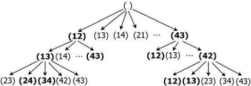
Fig.2. An example of a solution graph

The top of the graph is here the beginning t =0.

The next level t=1 represents a few possible variants of slots, i.e. (12), (13), …. (43). It should be noted that the slots (12) and (21) are different because train arrangement is important. For example, the train 2 has to unload containers to the staging area (which is considered as the track 0 which is closer to the track 1) and therefore it makes sense to place the train 2 to the track 1, which means that the slot (21) has a lower cost compared to (12).

Having generated all P = 12 possible slots K1 , the beam search procedure selects BW=2 slots/nodes with the best value of (1) for expanding. Other slots/nodes are excluded from further consideration. Let’s assume that we selected slots (12) and (43).

• IV. Computational Results

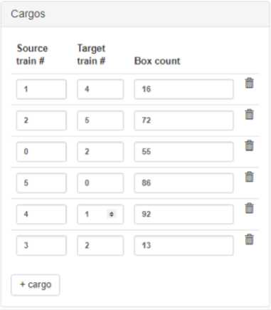
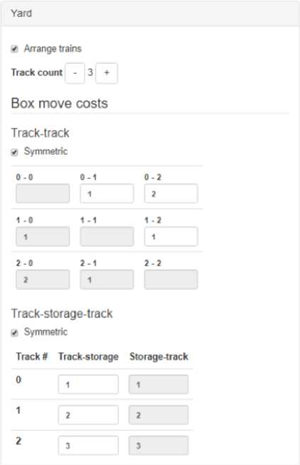
We implemented the solution algorithm in Python 2.7. A developed application is available online at Please take a look at screenshots of an example of input data and its solution in Figs. 3, 8, 9, 10.

Computational experiments were carried out to show how train arrangement impacts a solution quality and time. We generated a bunch of test instances. Every instance is a combination of following input parameters:

• •    9 options of a train count N =6,7, … ,14;

• •    4 options of a track count G =2,3,4,5;

• •    4 options of a track-track move cost:

c_pq = cost_coef * p - q , cost_coef = 1,10,50,100;

• •    5 various numbers of the target trains for each

train: when each train carries containers for 1,2,3,4,5 other trains; in other words, a various sparseness          of          a          matrix

N

• A :     A = 1,2,3,4,5, j = 1, 2... N . Let us denote

ij i=1

this parameter as cargos_per_train .

Objective weights were taken equal for all instances α ₁ = α ₂ = α ₃ = 1

We solved each of 9*4*4*5=720 instances twice: without train arrangement (solving only the level 1 issue described in [4]) and with train arrangement (solving also the level 2). For every instance, we calculated a relative time increase and a relative cost decrease of the solution with arrangements compared to the solution without arrangements:

cost_decrease = (c 1 -c 2 )/c 2 ,             (8)

time_increase = (t ₂ -t ₁ )/t ₁               (9)

where c 1 and c 2 determine values of the expression (1) for the solutions with and without arrangements; t 1 and t 2 define the solution time for the solutions with and without arrangements respectively.

One can find a full set of the solution data at

We have analyzed in what way each described input parameter may impact both the time increase and the cost decrease. Results are depicted in Figs. 4-7. Y-axis in all diagrams contains logarithms of cost_decrease and time_increase (y=lg cost_decrease, y=lg time_increase), while X-axis contains values of a specific input parameter.

The diagrams show that G and cargos_per_train directly impact both the cost decrease and the time increase while n generally impacts the time increase and cost_coef does not seem to impact either the time increase or the cost decrease.

Solution

Trains

• 6 Limit max slot count

Criteria weights

Criteria 1 • revisited trains count

Criteria 2 ■ split moves cost (trackstorage and storage track)

Criteria 3 ■ direct moves cost (track-track)

Solution time limit, seconds

Solution method

O Exact solution

• • Use beam search heuristic

Beam width

Train count - 6 +

Train # Earliest arrival slot # Latest departure slot #

• ⁰          1                      3

• 1                           Not limited

Not limited                 3

Fig.3. A screenshot of the developed application (input data)

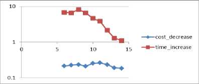
Fig.4. cost_decrease and time_increase (y axis) for various N (x axis)

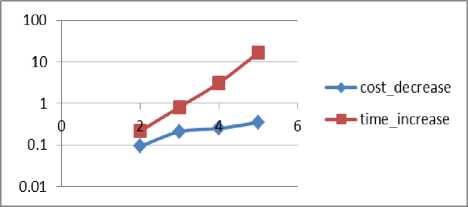
Fig.5. cost_decrease and time_increase (y axis) for various G (x axis)

Fig.6. cost_decrease and time_increase (y axis) for various cost_coef (x axis)

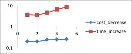
Fig.7. cost_decrease and time_increase (y axis) for various cargos_per_train (x axis)

• V. Conclusion

This article solves the second level of the transshipment yard scheduling problem, which includes assignment of the trains to the certain tracks.

The mathematical model and the solving method have been given for the described problem.

The article also describes TYSP in terms of the combinatorial optimization instead of using Boolean variables.

In computational experiments, we figured out that the solving problem for the second level allows decreasing the total schedule cost. However, more computational time is required to arrange the trains to the tracks.

The algorithm of the train arrangement could be improved in order to decrease computational time.

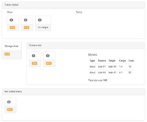
Fig.8. A screenshot of the developed application (its solution for the second slot)

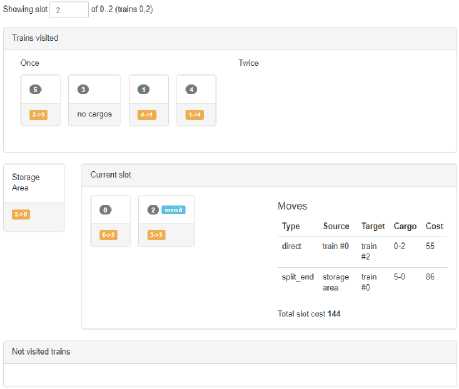
Fig.9. A screenshot of the developed application (its solution for the third slot)

View solution

Bestschedis $423:[(train #5, train #2, train #3)($171), (train #1. train #4)($108). (train #0. train #2)($144)]. Solution took 0 145433115005s 24 scheds generated

• • Progress

О Finish

Showing slot о of 0 .2 (trains 5,2,3}

Trains visited

Once                                             Twice

Current slot

Moves

Type      Source Target  Cargo Cost split_begin train #5  storage  5-086

direct       train #2  train #5  2-572

direct        train #3  train #2   3-213

Total slot cost 171

Not visited trains

ООО

Fig.10. A screenshot of the developed application (its solution for the first slot)