Selection of Optimum Rule Set of Two Dimensional Cellular Automata for Some Morphological Operations

Published Online November 2015 in MECS DOI: 10.5815/ijitcs.2015.12.06

Cellular Automata is also called systems of Finite Automata, i.e. Deterministic Finite Automata (DFA) arranged in an infinite, regular lattice structure [4]. In cellular automata state of a cell at the next time step is determined by the current states of a surrounding neighborhood of cells along with its own state and is updated synchronously in discrete time steps.

Formally, a (bi-directional, deterministic) cellular automaton is a triplet

A = (S; N; δ)                   (1)

Where, S is an non-empty state set, N is the neighborhood system, and

δ: S ^N → S                    (2)

is the local transition function (rule).

Due to simple structure and its property to model the complex systems, cellular automata has attracted various researchers from different areas. Cellular automata primarily announced by Ulam[1] and Von Neuman [2] in 1950’s with the purpose of obtaining models of biological self-reproduction and also discussed in the book of Wolfram ’A New Kind of Science’[3]. Now a day’s Cellular Automata became very popular because of its diverse function and utility as a discrete model for many processes. Cellular automata make up a very important class of completely discrete dynamical systems. Cellular Automata also provide a concept for computational automata.

Commonly used neighborhood systems are the von Neumann and Moore neighborhoods.

• A.    Von Neumann Neighborhood

A diamond shaped neighborhood that can be used to define a set of cells surrounding a given cell (x0, y0) that may affect the evolution of a two dimensional cellular automaton on a square grid. The von Neumann neighborhood of range r is defined by the equation 3.

N x0 ,y0 = {(x, y): |x - x 0 | + |y - y 0 | ≤ r}       (3)

The von Neumann neighborhood is illustrated in Fig 1.

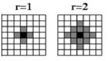
Fig. 1. Von Neumann Neighborhood

• B.    Moore Neighborhood

A square-shaped neighborhood that can be used to define a set of cells surrounding a given cell (x0, y0 ) that may affect the evolution of a two-dimensional cellular automaton on a square grid. The Moore neighborhood of range r is defined by the equation 2

N x0, y0 = {(x, y): |x - x 0 | ≤ r, |y - y 0 | ≤ r}      (4)

Moore neighborhoods is illustrated in Fig. 2

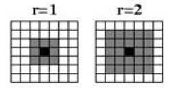
Fig. 2. Moore Neighborhood

• C.    Application of Cellular Automata

Some applications of cellular automata in modeling, controlling and analyzing of the behavior of complex are: The Games of Life [5], biological systems [6], Cellular automata in environmental system and ecological system [7], [8], CA in edge deduction [9], [10], [11], Cellular automata in the traffic system [12], CA in image processing [13]. Cellular automata in machine learning and control [14] and CA in cryptography [15].

Digital image processing(DIP) has very wide applications and almost all of the technical fields are impacted by DIP and it plays an important role in real life applications such as traffic analysis [32], satellite television, computer tomography and magnetic resonance imaging as well as in areas of research and technology such as biological information systems and astrophysics[16].Also it is used in Image sharpening and restoration, feature selection[31], Medical field, Remote sensing, Transmission and encoding, Machine/Robot vision, Color processing[30], Pattern recognition, Video processing, Microscopic Imaging etc.

Cellular automata are used in various image processing tasks such as image filtering in a better way than some existing filters in denoising process [17], [18], connected set morphology thinning and thickening of images [17], edge detection in digital images that provide boundaries of images[19], image segmentation which is an integral part of image processing applications like medical image analysis and photo editing[20], [19] and in Image Enhancement because of its dynamic behavior[21]. The advantage of cellular automata is that it provides simplicity in complexity i.e. though each cell has an extremely limited view of the system (just its immediate neighbors) and each cell generally contains simple rules, the combination of an array of cells with their local interaction leads to more sophisticated emergent global behavior of the system. This paper concentrates on the selection of the set of rules among the all possible combination of two dimensional cellular automata rules for the thinning and thickening process with their applications in different fields.

• II.    Optimization of Cellular Automata Rules

Cellular automata rule optimization is basically used to select the best possible rule set, among the all possible combination of rules, to perform the particular task, such as performance of cellular automata in image processing like- calculating distance features, Template Matching, noise filtering, thinning thickening, Image Sharpening, Simple Object Recognition using rule sets which provide specific operations to their states at each step of time.

• A. Related Work

To find out the optimum rule set, feature selection is acquiescent and can be performed using branch and bound algorithms [22]. In automatically optimization of rules most of the researchers focus in the density classification problem[20] that is recognized as a standard for exploring cellular automata rules with universal properties. Some authors further applied standard genetic algorithm (GA) for learning rules [20] [23]. A standard genetic programming platform is used in learning and training of cellular automata[24]. There are various feature selection methods that were introduced also consider GA and SFFS (sequential floating forward search)[24], [25], [17], where SFFS have better characteristics over the GA approach. Rule set automatically generated by evolutionary algorithms but probably this procedure was applied to artificial problems like- Majority Problem or for boundary detection in binary images[26], [27]. It depends on a rule set produced exact target output by increasing the size of neighborhood [28]. A form of hill climbing and backtracking algorithms also used to identify the rules. To optimize the cellular automata rules for image’s thinning and thickening process Paul Rosin[17] has been used root mean square(RMS) error criterion and Hausdorff distance error measures with SFFS procedure as objective function. But this approach did not produce satisfactory results and produced some lines in fragmented way. Fragmented problem overcame by an algorithm and two cycle cellular automata to produce better results in learning of rules[17].

• III.    Optimization of Cellular Automata Rules for Image Thinning and Thickening

Thinning and Thickening words come under the morphology operations that refer to form and structure; in computer visualization it can be used to refer to the shape of a region.

Thinning algorithms on binary images have a long history in image processing, because of their value in deriving higher representations (and compressed encodings) of the information in a bitmap. Thinning is a procedure to remove selected foreground pixels from binary images like erosion or opening. It is normally applied to binary images and produces another binary image as output. It can be used for several applications, but is particularly useful for skeletonization.

Thickening is a morphological operation that is used to breed particular regions of forefront pixels in binary images, that could be seem as dilation or closing. Basically Thickening process only applied to binary images, and by this it produces another binary image as output. The thickening operation is related to the hit-and-miss transform, There are various applications in image processing where thinning and thickening are used for different purposes as- Thinned images possess a subset of the original information that is useful for applications such as segmentation, feature extraction, vectorization, and pattern identification and thickening includes determining the approximate convex hull of a shape, to study any disease growing cell in spreading manner and determining the skeleton by zone of influenced region.

• IV.    Methodology

In this paper the binary images are considered i.e. cells have two states(white or black) and Moore neighborhood is considered in which the cells are eight ways connected and fixed value boundary conditions are applied which means transition rules are only applied to non boundary cells. The initial cell values are considered as the pixel values of the input image. As the Moore neighborhood is considered there are 28 rules are possible which are reduced to 51 by considering the 450 rotational symmetry and bilateral reflections [17]. Now the aim is to find the rule or set of rules among these selected 51 rules which provides the best thinning and thickening of the given image. Before applying the rules, the thinning and thickening of input image is obtained by the standard function bwmorph() available in the MATLAB and the resulting images are saved for the further references.

In order to select the best rule set for thinning of white portion, first the 3 x 3 neighborhood pattern of rule, as shown in Fig. 3, is compared with the 3 x 3 neighbors of the current pixel of input image. If both are not same then the central pixel is inverted in case of central white pixel. This operation is performed for all white pixels of the image. Each rule among 51 rules is applied at one time and the resulting image is compared with the image obtained by the standard function bwmorph(). Then the misclassification error[29] has been consider which is best suited for the classification of the thinned(thickened) white portion with standard function and rule set. The misclassification error is defined as

|B ∩ B | + |F ∩ F | error = 1 - ^{O      T      O      T}          (5)

B O + F O

Where, Fo and Bo shows the white and black pixels of the image obtained by the cellular automata rule whereas F T and B T are the white and black pixels of target image obtained by the standard function.

0	0	0		1	0	0		0	1	0
0	1	0		0	1	0		0	1	0
0	0	0		0	0	0		0	0	0
Rule 1				Rule2				Rule 3
1	0	0		0	1	0		0	1	0
0	1	0		0	1			0	1	0
0	0	1		0	0	0		0	1	0
Rule?				Rules				Rule 9
1	1	0		1	1	0		1	1	0
0	1	0		0	1	0		1	1	0
0	1	0		1	0	0		0	0	0
Rule 13				Rule 14				Rule 15
0	1	0		1	1	1		1	1	1
0	1	1		0	1	1		0	1	0
0	1	0		0	0	0		0	0	1
Rule 19				Rule 20				Rule 21
1	1	0		1	1	0		1	1	0
0	1	1		1		0		0	1	0
1	0	0		0	0	1		0	1	1
Rule 25				Rule 26				Rule 27
1	0	1		0	1	0		1	1	1
0	1	0		1	1			0	1	1
1	0	1		0	1	0		0	0	1
Rule 31				Rule 32				Rule 33
1	1	1		1	1	1		1	1	0
0	1	0		0		0		0	1
0	1	1		1	0	1		0	1	1
Rule 37				Rule 38				Rule 39
1	1	1		1	1	1		1	1	1
0	1	1		0	1	1		0	1	1
0	1	1		1	0	1		1	1	0
Rule 43				Rule 44				Rule 45
1	1	1		1	1	1		1	1	1
0	1	1		1	1	1		1	1	1
1	1	1		0	1	1		1	1	1
Rule 49				Rule 50				Rule 51

1	1	0		1	0	1		1	0	0
0	1	0		0	1	0		0	1	1
0	0	0		0	0	0		0	0	0
Rule 4				Rule 5				Rule 6
1	1	1		1	1	0		1	1	0
0	1	0		0	1	1		0	1	0
0	0	0		0	0	0		0	0	1
Rule 10				Rule 11				Rule 12
1	0	1		1	0	1		1	0	0
0	1	0		0	1	0		0	1	1
0	0	1		0	1	0		0	1	0
Rule 16				Rule 17				Rule 18
1	1	1		1	1	0		1	1	0
0	1	0		0		1		0	1	0
0	1	0		0	0	1		1	1	0
Rule 22				Rule 23				Rule 24
1	1	0		1	1	0		1	1	0
0	1	0		1	1			0	1	1
1	0	1		0	0	0		0	1	0
Rule 28				Rule 29				Rule 30
1	1	1		1	1	1		1	1	1
0	1	1		0	1	1		1	1	1
0	1	0		1	0	0		0	0	0
Rule 34				Rule 35				Rule 36
1	1	0		1	1	0		1	1	0
0	1	1		0	1	1		1	1	1
1	0	1		1	1	1		0	1	0
Rule 40				Rule 41				Rule 42
1	1	1		1	1	1		1	1	0
1	1	1		0	1	0		1	1	1
0	1	0		1	1	1		0	1	1
Rule 46				Rule 47				Rule 48

Fig. 3. Rule Set under Consideration

To compute the rule set for the thickening of the image the same procedure is used for the central black pixel i.e. if the central pixel is black and the encoded neighborhood pattern does not match with the encoded rule then the central pixel is inverted.

Proposed approach is providing Thinning and Thickening of white region on different images taking the advantage of cellular automata rules. The current paper shows only a subpart of test images to shown a fine visibility of the result.

Algorithm 1 Algorithm for Thining by Cellular Automata Rules

• 1:    PROCEDURE CA_THIN(A)

• 2:    Input : image A

• 3:   m ← 1

• 4    :      B ← A       // Save image A secondary image B

• 5:     E ← bwmorph(B) // thin the images by standard function bwmorph(),

• 6:     repeat

• 7:       C ← B

• 8:         For every pixel C[i,j] and Rule number = m

• 9:          begin

• 10:                S1 ← 3 × 3 neighbors of C[i][j].

• 11:               S2 ← 3 × 3 matrix of Rule m

• 12:                    if C[i, j] = white and S1 != S2 then

• 13:                         B[i, j] ← Invert (C[i, j])

• 14:          end for

• 15:     error[m] = 1 - |Bo ∩-BT | + |Fo ∩ FT |

Bo + Fo

• 16:         m ← m+1

• 17:    until m = 51

Algorithm 2 Sequential Floating Forward Search

• 1:    procedure SFFS

• 2:    Step 1:

• 3:    Y ← { ϕ}

• 4:    Step 2:

• 5:      Select the best feature

• 6:    x+ ← argmaxJ (Zk + x) | x ∉ Zk

• 7:    Zk ← Zk + x+

• 8:     k=k+1

• 9:    Step 3:

• 10:     Select the worst feature

• 11:     x- ← argmaxJ (Zk - x) | x ϵ Zk

• 12:    Step 4:

• 13:     if J (Zk - x- ) > J (Zk ) then

• 14:        Zk ← Zk - x-

• 15:         k =k + 1

• 16:          Go to Step3

• 17:else

• 18:         Go to Step2

The proposed method is shown as the procedure CA_THIN in algorithm 1. The rules are referred in the procedure by the rule number. The rules are numbered from 1 to 51 in Fig. 3 from left to right and upwards down manner. The proposed algorithm is initialized by setting the value of m as 1, here m shows the rule number. To find the thinning of the white portion, only white portion of the image is considered. For every white pixel, the 3x3 neighbors of pixel is considered and it is matched with the rule selected. If the 3x3 pattern of the pixel does not match with the rule under consideration then the central pixel is inverted otherwise it remains unchanged. This is applied for whole white portions of the image. When the whole image has been processed the misclassification error shown by the equation 5 is computed and stored in an array of error, where index of the array shows the error found by the particular rule number. Note that the black portion of the image is not considered here.

In each step each image pixel should be processed in parallel. However, since it is used as sequential operation, repeated until the maximum number of pixels matched to the standard method, the processed pixels are stored in a secondary image C. At the end of every iteration this processed pixel is copied back to original image.

In order to find the thickening of the white portion the same procedure with slight change can be used. To find the thickening, the algorithm 1 is applied to the black portion of the image. It should be noted that the rules shown in Fig. three are only for central white pixels. For central black pixel the rules shown in Fig. 3 are inverted.

To find the optimum set of the rules the sequential floating forward search(SFFS) method is used. The SFFS is a deterministic search method which provide the effectiveness equivalent to the genetic algorithm (GA)[23]. The algorithm 2 shows the SFFS algorithm.

Let Yk denote the rule set at iteration and its score be J (Zk ). Here, It is defined by the result of the algorithm by applying the CA rule set to the input image and computing the fitness function. Step 1 show that the initial set is empty. In step 2 at each iteration, all rules are considered for addition to the rule set and only the rule giving the maximum score is added the resulting rule set. This process is repeated until no improvements in score are gained by adding rules. In step 3, each rule in rule set found in step 2 is removed to find the rule whose removal provides the resulting rule set with the improved value of objective function. As shown in step 4 if removal of the rule cause the better score of the objective function then it is discarded from the rule set and again next rule is tried for the deletion and process go to step 3. Otherwise, the process go to step 2 for the addition of new rule to the rule set.

• V.    Experimental Results

  Following experiments are performed by using MATLAB 2014a. Considering 51 rules, which are used to provide thin or thick images at different iteration. Aforementioned procedure has been implemented and one pixel thinned image generated by the function bwmorph() available in MATLAB has been considered for the comparison purpose. In order to train the rule set 20 binary sample images are carefully selected in such a way that the images contains all kind of shapes such as lines, circles, cones and some complicated structures. Then the rules are trained by using the objective f unction misclassification error with the thinned image by the SFFS method as described in the previous section. In all the images the trained rule set which gives the best thinning result is rule number 51 as shown in Fig. 4.

1		1
	1
1		1

Rule 51

Fig. 4. Rule learned for Thinning and Thickening

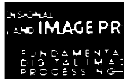
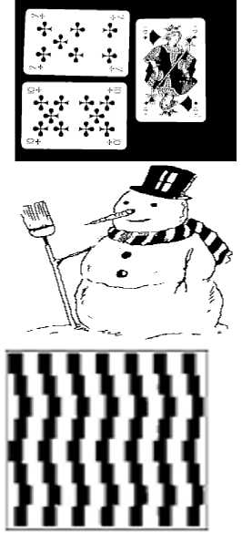
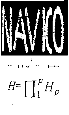
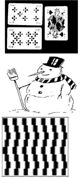
Fig. 5 shows the original input image. Then learned rule 51 is applied to these images which produced result in Fig. 6 that are compared to thinned images produced by standard function bwmorph() in shown in Fig. 7. Similarly, Fig. 8 and 9 show the results for thickening. It is also found that rule number 51 have the minimum misclassification error for the thickening operation and the images of Fig. 8 shows the result of the thickening performed by the rule 51 and Fig. 9 shows the thickening result of bwmorph(). Besides these images experiment of optimization of cellular automata for thinning and thickening of images using best rules set at which minimum misclassification error is occurred in corresponding to standard function is done on several other images and in all the cases the rule number 51 shown in Fig. 4 is found best for the thinning and thickening operations.

Since the proposed algorithm is simulated on the sequential machine in MATLAB 2014a the time required to find the result is high. But once the rule set is trained for the thinning and thickening, then it is quite easier to apply the trained rule set to the images to find the desired result.

TEST

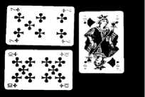
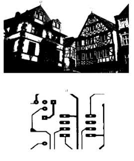
Fig. 5. Original Images

ЙЙ1Й

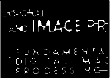
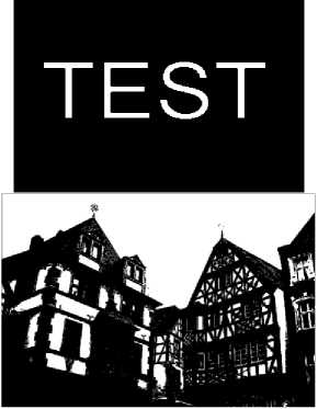
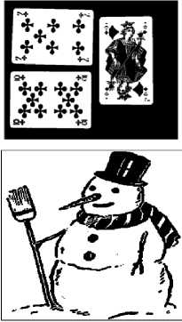
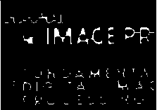
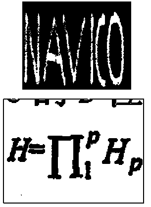
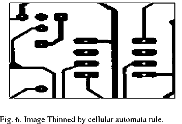
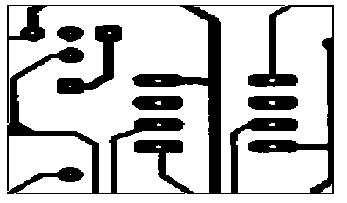
Fig. 7. Image Thinned by Standard Function

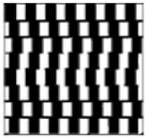
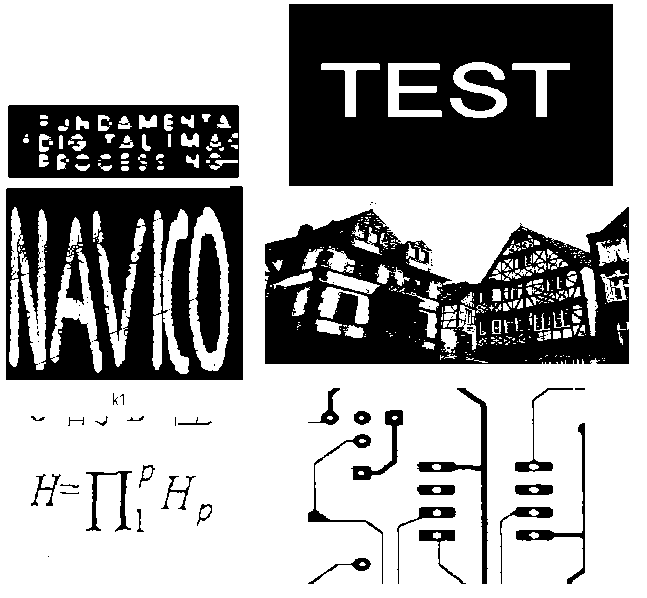
Fig. 8. Images Thickend by cellular automata rule.

;s^g4u

. ив IMAGE PR

*i^34U

«IMAGE PR

: j h C- 4 М E 4 T A

•c-ю T4i 1ЫД-: е»5С:И ч->-

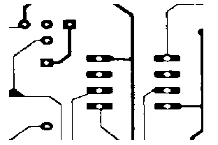
Fig. 9. Images Thickend by standard function.

• VI.    Conclusion and Future Work

Results for the thinning and thickening of binary images through cellular automata rules are encouraging. The resulting rule sets provides comparable thinning and thickening as compared with the standard function bwmorph().Implementation and use of cellular automata rules is easier and straight forward as compare to other methods and also the size and the dimensions of images does not affect the complexity of the cellular automata. It is also required to mention that the aim to use the cellular automata is to provide simplicity to solve the complex processes which is fulfilled in our experiment and clearly depicted in the results section. As the work presented in the paper is limited in thinning and thickening with the use of the sequential floating forward search method. It can be extended for some other morphological and image processing operations.