Self-Load Balanced Clustering Algorithm for Routing in Wireless Sensor Networks

Published Online September 2017 in MECS

A Wireless Sensor Network is a collection of tiny electronic devices comprising sensors and transceivers. Sensors have the ability to monitor physical and environmental conditions. Typically, WSNs are unattended after deployment and the sensors have limitations on battery power, connectivity, storage and infrastructure [1]. The development of WSN was initiated by military applications (battlefield surveillance) [2]. WSNs are now implemented in commercial applications like human health monitoring, factory automation, environmental monitoring for temperature, lighting, humidity, and so on. Sensor networks have high reliability on scaling, as they support self-configuration and self-management [3]. In WSN, sensors’ energy outage is seen as a major network failure, where sensors are the network’s primary element and they are battery operated. Due to being unattended, recharging or replacing sensor’s battery is very difficult and cost effective. So, designing energy-efficient communication structure in WSN is essential to prolong its lifetime. Among sensors’ operations, data transmission is a major energy consumer and the consumption rate is directly proportional to the communication distance (distance between sender and receiver). So, lowering communication distance between nodes could increase the network lifetime.

Clustering the network is the key solution for nodes’ energy conservation, as it has a hierarchical data collection mechanism. Clustering is a process of grouping sensors under a specific condition. A node from each group is selected as ClusterHead (CH) to employ cluster operations. Constructing CDS in a network is an efficient solution for network clustering [4–8]. Some graph terminologies relevant to CDS construction are given below.

Graph: A graph G is a pair of sets ( V , E ) , consists of a non-empty set V of vertices (nodes) and another set E whose elements are called edges (links), such that each edge e is identified with an unordered pair ( v , u ) of vertices.

Neighbour or adjacent node: Vertex v is adjacent to u , if there is an edge e , such that e = ( u , v ) .

Neighbour Set ( N ( v ) ) : Neighbour set of v is defined as N ( v ) = { u |( u , v ) ∈ E } .

Degree: The degree of a node v is the number of edges incident on v , and is denoted by deg(v) .

Maximum degree ( Δ ): The maximum degree of a node in graph G is Δ = max{deg(v) |v ∈ V(G)}.

Dominating Set (DS): A set D ⊂ V(G) a DS, if every node in V - D is adjacent to at least one node in D . Nodes in DS are called dominators, and particularly known as ClusterHeads (CHs) in network clustering problems. Nodes of V - D are called dominatees or cluster members.

Connected Dominating Set (CDS): If the graph induced by a subset DS is connected, then that DS is known as a Connected Dominating Set (CDS).

CDS size : The number of nodes in a CDS represents its size.

In CDS based clustering, each node in a CDS represents a CH that responsible for collecting data packets from cluster members, aggregate and transmit it to the base station [8]. Transmission rate depends on the number of CHs, so clustering a network with an optimal CDS size is essential to maximize the network lifetime. When CDS size is minimum, transmission rate decreases considerably. But, CHs suffer due to high data processing overheads that leading to rapid energy depletion. When CDS size is maximum, transmission rates increase extremely, thereby voiding the clustering benefits. So, this paper proposes a greedy CDS based clustering algorithm SLBC to construct an optimal number of clusters. The performance of the proposed algorithm is evaluated through simulation and compared with minimum sized CDS algorithm DGA-EBCDS and the maximum sized CDS algorithm GSTEB.

The rest of the paper is organized as follows: Section II reviews the related work. The network and radio model of the proposed algorithm is discussed in Section III. Section IV describes the problem statements and the proposed algorithm, SLBC. Section V presents the results and discussions of SLBC. Finally, Section VI concludes the paper.

• II.    Related Work

Many heuristic CDS based clustering algorithms are proposed in literature with different design perspectives [4 - 6], [9-11]. Typically, WSNs are modelled as a Unit Disk Graph (UDG). In such graphs, nodes are unit circles, where any two nodes are said to be adjacent, if and only if, they reside within the unit distance. As data transmission is a major energy consumer in WSNs, most current algorithms address the Minimum sized CDS (MCDS) to reduce global communication distances and transmission rates [12].

Typically, CDS construction algorithms are classified [13] into centralized and decentralized (distributed) algorithms. Centralized algorithms prefer a MCDS with higher performance ratio. Such algorithms generally need total knowledge of network topology. In 1998, two centralized greedy heuristic algorithms for a general graphs were proposed by Guha and Khullar [7]. The first algorithm constructs a spanning tree (T) by choosing a maximum degree vertex as root. In each step, an additional fitted-vertex is added into T. It has a performance ratio of2(H(5) +1), where 5 is maximum node degree. The second algorithm is an enhancement of the first and has two phases. The first phase constructs the dominating set and is connected using the Steiner Tree in the second phase. The performance ratio of the second algorithm is H(5) + 2 . Later Ruan et al., [14] proposed a one-step greedy approximation algorithm, which modifies the potential function of Guha et al., and obtains a performance ratio of (2 + ln5) . Misra et al. [15] presented a collaborative cover heuristic CDS construction algorithm that builds a Maximal Independent Set (MIS) using an effective coverage metric. Further, MIS nodes are connected as a Steiner tree by identifying Steiner nodes. This algorithm has a performance ratio of (4.8+ln5) |opt|+1.2, where |opt| is the size of any optimal CDS in the network.

Das et al. [16] proposed a Steiner tree based algorithm called Pseudo-dominating Set Construction And Steiner Tree Spanning (PSCASTS), that builds the CDS in three stages. In the first stage, PSCASTS greedily constructs a pseudo-dominating set offering MIS with minimum cardinality. The second stage forms a Steiner tree by choosing Steiner nodes that connect more MIS nodes. Finally, in the third stage redundant CDS nodes are pruned. PSCASTS retains a performance ratio of collaborative cover heuristic proposed in [15]. Another Energy efficient MCDS construction algorithm (E-MCDS) proposed by Tang, Qiang, et al. [17], constructs the CDS in two stages: the CDS construction stage and the pruning stage. Further CDS construction divided in to CS construction stage and DS construction stage. Dominators are selected in CS stage and the remaining uncovered nodes by CS stage is covered by DS stage. In pruning stage, E-MCDS removes the redundant dominators in CDS that reduces the CDS size. As, finding MCDS in UDG is a NP-hard problem [18] and constructs the cluster with more members, the lifetime of the CHs is shortened due to its additional data processing. Therefore, centralized-CDS algorithms are unfeasible for use in conducting CDS in WSNs. Hence, distributed algorithms are a better option for CDS construction as they prefer the metric of CDS construction process instead of a small sized CDS [19]. A metric may be a transmission rate and node’s proximity.

Aziz et al. [20] proposed a Single-Phase Single Initiator (SPSI) Algorithm for distributed energy aware CDS construction. SPSI is an enhanced form of MPRs (Multi Point Relays) heuristic approach proposed by Qayyum et al. [21] that aims to reduce the CDS size. In this approach, each dominator chooses a set of connectors from its first hop neighbours, thereby covering the maximum two-hop neighbours. The chosen connectors become CHs and continue connector’s selection from its neighbours. So, nodes should be aware of their 2-hop neighbours. It has O(3AC+3A) time and O(n) message complexity, where A is the maximum degree of a node. As maximum degree node has higher probability on dominator selection, dominators in SPSI are suffer heavily due to early energy depletion. DGA-EBCDS algorithm similar to SPSI was proposed by Kui et al. [22] to reduce CDS size. It has two phases; the MIS is constructed in the first phase, and nodes in MIS are connected using connectors in the second phase. MIS construction is prioritized by the node’s degree and residual energy. The connectors are chosen from the neighbours of MIS nodes, which have more residual energy and better connection between them. The algorithm chooses a maximum of two connectors to connect adjacent MIS nodes (i.e. CHs). In DGA-EBCDS, network lifetime is achieved by choosing higher residual energy nodes as CHs and by constructing the data collection tree. However, it includes more intermediate nodes (connectors) that increase the transmission rate unnecessarily. It also fails to distribute the nodes among CHs. This leads to maximum degree nodes die earlier as it has higher residual energy when choosing it.

Han, Zhao, et al proposed a General Self-Organized Tree-Based Energy-Balance (GSTEB) routing protocol [23] to construct a cluster backbone. In each round, the base station selects a maximum energy node as root and other nodes are choose one of its neighbours as CH, which is closer to the root. If there are no such neighbours, the node selects the root as its CH. GSTEB is discussed in two types of radio models. The first radio model implements a data fusion technique and only the root can directly communicate with the base station. In the second radio model, data cannot be fused and also more nodes can communicate directly with the base station. As GSTEB constructs multi-branch with a chain like clustering, node’s energy consumption is significantly increased, due to higher data reception and transmission, specifically the nodes that closer to the root.

Due to additional data manipulation, CHs premature death is a prominent issue in clustering algorithms. Recent algorithms to offset this, periodically perform reclustering. But, recurrent re-clustering generates additional control message overheads, leading to nodes unnecessary energy depletion. During re-clustering, data transmission is suspended, which is a substantial issue in time critical applications. This paper constructs well-balanced CDS for network clustering and proposes an on-demand rotation scheme for re-clustering.

• III.    Network and Radio Model

The proposed network model adopts some of the following assumptions.

The ‘ n ’ number of homogeneous and static sensor nodes are distributed in a two dimensional plan with compatible density, to ensure maximum connectivity and coverage. So, sensors have same transmission and sensing capability and the maximum transmission range of a node is denoted as R . Nodes are identified using a sequence of numbers (1, 2...n) called node ID. Nodes have a unique battery source with same amount of energy (in joule) during installation. It is assumed that the network is unattended and primary node failure is due to power depletion. Nodes are capable of dynamic transmission range adjustments. When two nodes are neighbours, they must reside within each other’s transmission range ( R ) . Nodes are unaware of the geometrical information of their neighbours. But, it can compute the approximate distance of neighbours using

Received Signal Strength Indicator (RSSI) [24].

The proposed algorithm uses the first order radio model as in [22, 23, 25] where radio transmitter and receiver circuitry energy consumption are E elec = 50 nJ / bit and transmitter amplifier dissipate is considered 10 pJ / bit / m ² for the free space propagation model ( £ fs ) ( d ² path loss) and 0.013 pJ / bit / m ⁴ for the two-ray ground model ( £ _mp ) ( d ⁴ path loss). Thus, l bit message over distance d , energy consumption to transmit e ( l , d ) is calculated as

E tx ( l , d ) 4

+ 1. £ fs . d ² , if d <  1

+ 1. £ mp . d 4 , if d >  1

^{l . E} elec . E elec

Energy consumption to receive this message is

E RX ( l ) = l . E elec                    (2)

Communication between two nodes is undertaken through IEEE 802.15.4 standard wireless radio full duplex method.

• IV.    Proposed Slbc Algorithm

The proposed SLBC algorithm is described Setup and steady state phases. The setup phase describes weighted CDS construction and the steady state phase describes data collection and the proposed on-demand rotation scheme.

• A.    Weight (W) calculation

Nodes weight calculation to become a CH is based on three properties; Reduced Degree ( deg_r ) , coverage Integrity ( I ) and Energy cost ( E_C ).

Reduced Degree (deg_r ): The reduced degree of a node represents the number of its uncovered neighbours. This property is adopted from CH selection criteria of the current algorithm [7]. Let S be a set of nodes dominated by current CDS. If N ( v ) is a neighbour set of node v, then the reduced degree of v is calculated as:

deg r ( v ) = | { u : u e N ( v ), u t S }| (3)

Selecting the maximum reduced degree node’s as a CH, reduces CDS size considerably, as it forms cluster with more uncovered nodes.

Coverage Integrity ( I ): Coverage integrity is a measurement to what degree a node can dominate the uncovered neighbours of its co-members. The Higher precedence of nodes coverage integrity in W estimation increases the node’s dissemination efficiency. Hence, CH’s premature death caused by communication overheads is reduced considerably. Nodes, coverage integrity increases the probability of sensed data within cluster members being highly correlated, thereby increasing efficiency of data aggregation. It also reduces the energy consumption of CHs, due to complex data aggregation processes. But, it could include additional nodes in the CDS, when a node with more coverage integrity and lesser reduced degree than competing nodes is chosen. Let node v be dominated by u, then coverage integrity of v with respect to u is defined as

I(v, u) =

N(v) ⁿ1 U { ^fck ^e N(i),k ^ ^S } [ i e N(u)

where N(v) and N(u) are a neighbour set of v and u respectively.

Energy Cost (E ): Let E_r ( v ) be the residual energy of node v at round r and E_i ( v ) its initial energy. Then the energy cost of v is defined as

E c (v) =

E r (v)

E i (v) - E r (v)

Energy Cost of nodes lead to choosing a CH with maximum energy. Let u be the CH of node v . Using equations (3), (4), and (5), weight of v to become a CH is formulated with respect to u as

W ( v , u ) = ( a x deg r ( v ) ) + ( ^ x I ( v , u ) ) + ( y x E C ( v ) ) (6)

a , в and у are balancing factors ( a + в + Y =1), and are valued based on application perspectives. Weight estimation of the proposed SLBC algorithm does not consider the distance between CHs. The primary objective of SLBC is to construct an optimal CDS and so chooses a CH with more uncovered neighbours. An attempt is made to reduce the distance of CHs that increase CDS size as a node closer to CH will have minimum chance of having more uncovered neighbours.

• B.    Parent Fitness cost

As nodes can have more CH neighbours, SLBC disseminates them among clusters via an independent node distribution scheme, where nodes are distributed through use of a defined parent fitness cost. It is a CH’s quality measurement estimated by a node using Euclidian distance and the approximated lifetime of the corresponding CH. As data transmission consume much energy and as such consumption is directly proportional to the distance among nodes, decreasing transmission distance between the nodes and CH significantly lowers the nodes energy depletion [26]. So, the nodes are prepared towards the CH with minimum distance. Let u be a CH and v be a CH neighbour of u , residing in the communication path between u and the base station. Let d ( u , v ) be distance between u and v . The estimated lifetime of u is denoted as T ( u ) and defined as

T ( u ) =

E_r ( u )

E_T x ( l , d ( u , v )) + ( E rx ( l ) x deg_r ( u ) )

Consideration of the approximated lifetime of a CH, aids energy efficient node distribution. Let w belongs to N(u) , then the parent fitness value of u regarding w is defined as:

F ( u , w )

^ 1

d ( u , w )

+ ( ^ 2 x T ( u ) )

^ , ^ are balancing factors which lie between 0 and 1, and whose sum is 1.

• C.    Clustering process

The proposed algorithm uses depth first tree traversing mechanism with node colouring procedure to construct a CDS, where ‘ black ’, ‘ grey ’, and ‘ white ’ represent the CHs (dominators), cluster members and uncovered nodes respectively. A node is covered, it must be neighbour of a CDS node. All nodes are coloured ‘ white ’ when deployed. The base station selects a node from r radius as root (initial CH), say u , with maximum weight. Further, u is added to the set CDS and coloured ‘ black ’. When u is selected as CH, it broadcasts an elected message to neighbours with the following parameters; { ID ( u ), E_r ( u ) , deg_r ( u ) )}. Let v be a neighbour of u that receives the message. Then it sends a response message to u with the following parameters:   { ID

(v) , E_r ( v ), Js e {0,1}, W(v, u) } . Here, Js notifies whether v will join (1) the cluster of u or not (0). It is defined as

1 1    colour ( v ) ^ ' white' or if F ( v , u ) >  F ( v , w )

Js = ^

I 0 otherwise

After receiving the response from each neighbour, u finalizes the cluster members according to the status of Js flag. The white neighbours of u are coloured ‘ grey’ . Subsequently, u selects one of the ‘ grey’ neighbour with maximum weight, say v , as a succeeding CH and is coloured black . Similar to u , v sends an elected message to neighbours and forms a cluster according to the joining status of the neighbour’s response. Further, white neighbours of v coloured ‘ grey’ and v starts selection of the next CH. This process continues until all the network nodes are coloured ‘ grey’ or ‘ black’ . A set of black nodes represents the CDS. Each CDS node form one cluster using its cluster members. After clustering, nodes reduce their transmission range according to the distance of its CH. The procedure of the proposed algorithm is represented in algorithm 1. The fitness based CH selection procedure is denoted as Independent Node Distribution (IND) and described in algorithm 2.

• D.    Steady State Phase

After successful clustering, a TDMA (Time Division

Multiple Access) schedule is prepared by the base station. Further, nodes transmit their data to corresponding CH in a specified time slot. CHs collect data from cluster members, aggregate and transmit it to the base station directly (when the base station is a one-hop distance) or through intermediate CHs in the clustering hierarchy. One complete data collection by the base station is referred as a round. As premature death of CHs is a prominent issue in the design of clustering protocols, the current algorithms perform re-clustering at every round to overcome this. However, this recurrent re-clustering exponentially increases control message overheads for cluster formation, which shortens nodes lifetime significantly. During this phase, data transmission is interrupted, which is a precarious issue in time critical applications [27]. Therefore, SLBC proposes a new on-demand rotation scheme, which performs re-clustering when the residual energy of any CH is reduced to certain level of its cluster members.

On-demand rotation scheme: Let u be a CH and N ( u ) be a set of cluster members of u , then u sends a special beacon message to the base station to initiate reclustering when the following condition is satisfied.

£ E r ( k )

( E, ( u ) - E ( u )) <    '----x o           (10)

I        r         |Nd(u)| where Er(k) represents residual energy of k at round r and o (0 < o < 1) is an energy threshold variable. As cluster members transmit sensed data to CH, the current residual energy of cluster members is estimated based on the transmission cost. Let rc be the current round and ri be the round of the last successful (re-)clustering. Let Ei (k) be the residual energy of k at round ri , Er(k) at rc which is calculated as

E r ( k ) = E_t ( k ) - ( r c - r i ) E tx ( k )          (11)

c

E ( k ) is the transmission cost of one round. E_i ( k ) is collected by u when clustering. As nodes can find neighbours distance using the RSSI method, finding residual energy of neighbours does not need additional control messages. Whenever the base station receives this message from a CH, it initiates re-clustering by performing the setup phase. The setup and steady state phases are sequentially executed till the first node fails. The performance of the proposed algorithm is evaluated through simulation and the results described in section V.

• E.    Energy consumption Analysis of proposed algorithm per round

In each round, a node generates l bit of data and send it to the CH. Let u be the CH, consists of n cluster members and v, be the th ( i e {1,2,... л }) cluster member of u . Hence from Equation 1, the energy consumption for sending data from all the cluster members to u is expressed as

n

^E cm ^{( U} ) = £ ^{1 X} E elec + ^{1 X} ^ fs ^{X ( d ( U} , v i ⁾⁾² ,       ⁽¹²⁾

i = 1

Also from Equation (2), energy consumption of u for receiving and aggregating cluster member’s data is expressed as

E ch ( u ) = л ( l X E elec ) + ( л + 1)( l x E da ),       (13)

where E_DA represents the energy consumption to aggregate one bit of data. Since u also performs sensing operation, data of u is included in data aggregation. From Equations (12) & (13), total energy consumption for intra-cluster data collection is derived as

E collect ( U ) = E cm ( U ) + E cH ( U ), (14)

Let l ₁ be the aggregated data length of u and f_agg e (0,1) is the data aggregation factor [24]. Then l1 is calculated as

₁ _ l x ( л + 1) Ц =

^{( л x} f atggg ) ^{+ 1}

Further, u sends aggregated data to the base station through a multi-hop model. Let h be the hop distance of path from u to the sink in the proposed clustering structure. Then the total energy depletion for sending this l ₁ bit of data to the sink is calculated as

h

^E m _ hop ( ^U ) = ^l 1 £ ² E elec ⁺ ( ^ mp ^X d_BHopl       ⁽¹⁶⁾

i = 1

where d < R represents distance between two toHop adjacent CHs. Total energy consumption of the proposed algorithm per round is calculated from Equations (12), (14) and (16), and given as

| CDS |

^E perRound = £ [ E Collect ^{( u}i ) ⁺ E cm ^{( u}i ) ^{+ E}m _ hop ^{( u}i ) J , i = 1

Algorithm1SLBC( G(V,E) )

• ▻    Input :V ( G ), E ( G )

• ▻    set color (V ( G )) ^ ' white

• ▻    stk : T emporary stack initiallyempty

• ▻    top ^ 0

• ▻    CDS :initiallyempty

• ▻    N ( CDS ): Neighbour set of CDS

• ▻    Output : CDS ( G )

• 1 : Find u |max( F ( sink , u )), d ( u , sink ) <  R

• 2    : Set head ( u ) ^ ' sink'

• 3    : while top >  0 do

• 4    :  if color ( u ) ^ ' black ' then

• 5    :     push ( stk ( top )) ^ u

• 6 :      color ( u ) ^ ' black'

• 7 :    CDS <  u } u CDS

• 8    :     CallIND ( N ( u ), u )

• 9    :     top ^ top + 1

• 10    : end if

• 11 : W ^ 0, SelectCH ^ ' null'

  // W , SelectCH are temp variables

• 12    : for all v e N ( u ) - { CDS } do

• 13 :       Calculate W ( v , u )

• 14 :     if W ( v , u ) > W then

• 15 :        SelectCH ^ v

• 16 :        W ^ W ( v , u )

• 17    :     end if

• 18    :  end for

• 19    :  if selectCH then

• 20 :     head ( SelectCH ) ^ u

• 21 :     u ^ SelectCH

• 22    :   else

• 23    :      top ^ top - 1

• 24    :      u ^ stk ( top )

• 25    :   end if

• 26    : end while

• F. Time complexity of SLBC

The time complexity of each stack operations is O(1). The proposed algorithm uses the backtrack method to construct the clusters that performs maximum of |CDS| times push and pop operations. Hence the time complexity of the while loop is 2|CDS|. The algorithm repeats the statement finding the new dominator in the maximum of A times inside the while loop. So the maximum time complexity of the proposed algorithm is O (2 A | CDS |).

Algorithm 2 IND( N(u),u )

• 1    :£>r all w e N ( u ) do

• 2    : if color ( w ) ^ ' white then

• 3    :    color ( w ) ^ ' grey'

• 4 :   head ( w ) ^ u

• 5    : else

• 6    :  if F ( w , u ) >  F ( w , head ( w ) ) then

• 7 :     head ( w ) ^ u

• 8    :   end if

• 9    : end if

• 10    :end for

• V. Experimantal Results and Discussion

This section discuss the experimental analysis of proposed and compared algorithms (E-MCDS [15], DGA-EBCDS [22] and GSTEB [23]) in various network scenarios and aspects.

• A.    Simulation Setup

This section describes the simulation results and performance evaluation of the proposed algorithm in terms of CDS size, load dissemination, network lifetime, and efficient energy utilization. The obtained results are compared to the current clustering algorithms E-MCDS, DGA-EBCDS and GSTEB. The aforementioned network model (in section III) is used to construct network topology for experiments. To ensure a unified comparison, the compared algorithms uses the similar network setup and energy model. Results are obtained from 100 experiments on each algorithm with node densities ranging from 50 to 200. Parameters used in the experiments are shown in Table 1. A node’s initial transmission range is defined by Equation (18) as in [28], which estimates the minimum transmission range, thus ensuring full connectivity. Let N be the number of nodes in a network and L be a side of squared deployment region. The transmission range of a node is calculated as:

R = 2LL _x I log fC N N

Table 1. Simulation Parameters And Their Values

Network Deployment area Size	100X100, 200X200
Number of nodes	50 to 200
Base station/sink position	Middle of the Area of Interest
Data Packet size	4000 bits
Control packet size	200 bits
Energy Consumption for TX,RX	50 nJ
Energy for data aggregation (EDA)	5 nJ/bit/signal
Initial node energy	2 Joule
Sensors Communication Range	R

• B.    Clustering Structure

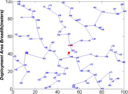
One of the main objectives of the proposed algorithm is to disseminate load among clusters. To show the superiority of the proposed algorithm on load dissemination, it is essential to evaluate the proposed cluster structure. Figures 1, 2, 3, and 4 show the sample clustering structure of the DGA-EBCDS, E-MCDS, GSTEB and proposed SLBC algorithm, respectively. DGA-EBCDS constructs CHs based on the node’s degree and does not perform load distribution. Hence, DGA-EBCDS suffers extremely due to uneven load dissemination of clusters, as shown in figure 1. As E-MCDS use reduced degree of nodes, it shows better distributed structure than the DGA-EBCDS. However, E-MCDS also fails to distribute the nodes among CHs. Thus, some CHs are suffered by higher cluster members, as shown in figure 2. The algorithm GSTEB constructs a tree structure based on the distance between the nodes and the base station. As branches are constructed like a chain of nodes, transmission rate and average communication distance between the nodes to the root increases significantly. But, the proposed SLBC algorithm employs IND process for distributing nodes among CHs, which is proved in figure 4. As DGA-EBCDS constructs the collection tree for data collection, average communication length of CHs in SLBC is slightly higher compared to DGA-EBCDS. But, this limitation is nullified when compared to the load dissemination improvement of the proposed algorithm.

• C.    CDS size

This section analyses the number of clusters constructed by E-MCDS, DGA-EBCDS and the proposed SLBC. Results are shown in figures 5 and 6, where figure 5 shows the CDS size obtained when the deployment area (L) is 100 m² and figure 6 shows the CDS size of the algorithms, when L is 200 m² . GSTEB constructs chain like tree structure, if each non-leaf node in the tree is considered as a CH, the number of clusters is enormous. So, GSTEB is not considered for CDS based studies.

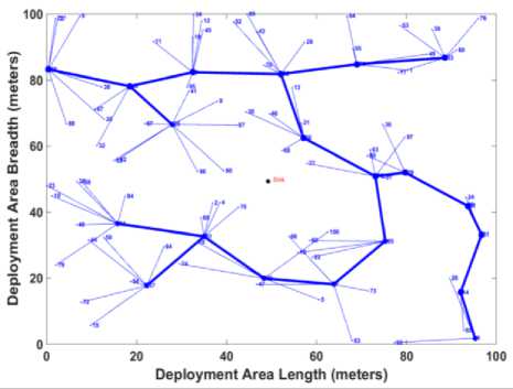
Fig.1. E-MCDS Clustering Structure

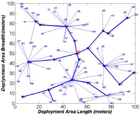
Fig.2. DGA-EBCDS Clustering Structure

Deployment Area Length(meters)

Fig.3. GSTEB Clustering Structure

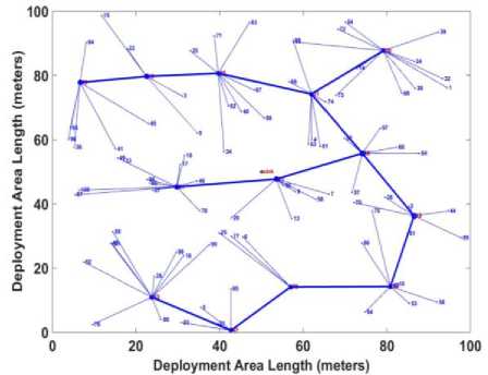
Fig.4. SLBC Clustering Structure

DGA-EBCDS selects higher degree nodes as CHs and connects those using common neighbours. Then, the size of CDS increases considerably due to more connecting nodes. However, as the proposed algorithm performs tree-based clustering, and as CHs are chosen based on nodes reduced degree, it ensures a smaller sized CDS than DGA-EDCDS, which is shown in figures 5 and 6. As like the proposed algorithm, E-MCDS also selects the CHs based on the reduced degree. But the DS construction stage of E-MCDS includes some more nodes into the CDS. Though, E-MCDS shows CDS size, which is very nearer to the proposed algorithm. As nodes transmission range is defined based on the network size and deployment area, nodes average degree is reduces when network size increases. Then the algorithms constructs more CHs to cover the entire network region. So, in figures 5 and 6 the size of CDS increases with network size and deployment region.

• D.    Load dissemination

Load dissemination of the proposed algorithm is evaluated based on the cluster density (number of nodes in a cluster) and size difference between maximum and minimum dense clusters. In each experiment, the number of nodes in the maximum dense cluster is obtained and the average of this result is used to analyses cluster density. The result is shown in figures 7 and 8 for two size of deployment areas 100 m² and 200 m² respectively. DGA-EBCDS selects maximum degree nodes as CH and does not perform node distribution among clusters. Hence, some CHs suffer by additional cluster members, where others have a minimum. In a worst case scenario, nodes in a dense cluster is equal to 30 percentage of network size, as depicted in figures 7 and 8. As E-MCDS selects the CHs based on the reduced degree, it reduced the number of nodes per CH. But, it’s not perform node distribution among CHs, so still the CHs are suffered by uneven load dissemination.

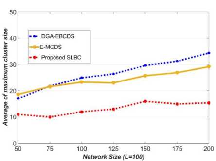
Fig.7. Comparison of average cluster size (L=100 m² )

The proposed algorithm uses the coverage density of the nodes is one of the prime factor for CH selection, which increases the efficiency of the IND process. So, nodes are evenly distributed among CHs. In figures 7 and 8, the proposed algorithm constructs a cluster with minimum nodes than DGA-EBCDS and E-MCDS for all network sizes. Figure 9 shows the size difference between maximum and minimum dense clusters when L is 100 m² . Among the compared algorithms, the SLBC shows the least members difference between the maximum and minimum dense clusters. Hence, it is proved that the proposed algorithm is superior to DGA-EBCDS and E-MCDS in terms of load dissemination.

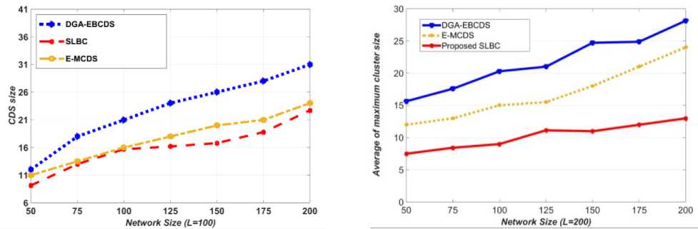
Fig.8. Comparison of average cluster size (L=200 m² )

Fig.5. Comparison of CDS Size when L=100.

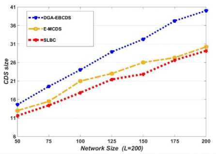
Fig.6. Comparison of CDS Size when L=200

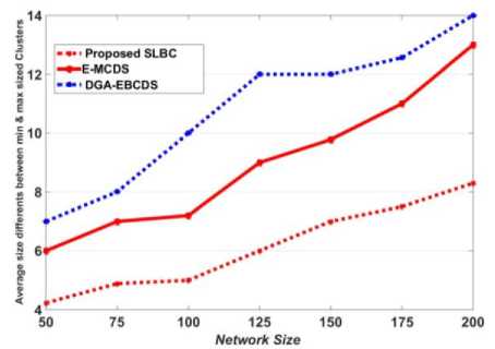
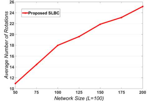
Fig.10. Average number of rotations by SLBC

• E.    Re-clustering overheads of SLBC

As the proposed algorithm performs on-demand rotation for avoiding early energy depletion of CH, average number of rotations per experiment is considered for analysing its re-clustering overheads. Figure 10 shows the average rotations yielded by the proposed algorithm SLBC against various network sizes, when L is 100 m² . As cluster density increases with network size, CHs experience higher energy depletion due to more data processing. So, the frequency of re-clustering is increases with the network size, as it is shown in figure 10. However, the percentage of rotations by SLBC against the number of its rounds is approximately 0.83%, which infers the re-clustering overheads of SLBC is insignificant.

• F.    Network Lifetime when first node dies

Network lifetime is analysed in terms of rounds. One round represents a complete cycle of data transmission from all the nodes to the base station. The number of rounds is calculated from the initialization of the network till the  first node dies. Figure 11 represents the comparison of network lifetime for the proposed and existing  algorithms in various network sizes.  The algorithm GSTEB builds a routing tree (Case1 in GSTEB) based on the distance between the nodes and the root node. So, almost all nodes in GSTEB participate in data forwarding, increasing the transmission rate exponentially. Due to more data transmission overheads, nodes experience undesirable energy depletion and energy is drained earlier. Moreover, the algorithm’s reclustering fails to distribute nodes energy consumption, as it is just used to change data flow direction. Also, during re-clustering nodes suffer by control message overheads. These limitations of GSTEB reduce the network lifetime considerably.

In DGA-EBCDS, CHs are severely suffered by uneven load dissemination, so it’s experience more data processing and die earlier. As DGA-EBCDS is not consider the intra-cluster communication distance for clustering, normal nodes have more probability to join with the far CH. As a result, it spends more energy for data transmission. For these reasons, DGA-EBCDS shows minimum network lifetime when compared to the proposed SLBC and GSTEB. The algorithm E-MCDS is concentrates to reduce the transmission rate by reducing CDS size, then the CHs in E-MCDS is heavily suffered by higher data processing and die earlier. But, it reduces the density of cluster through reduced degree based CH selection procedure, so it shows better lifetime than DGA-EBCDS.

The proposed SLBC algorithm selects CHs based on the defined weight factors, which leads to select the CHs with more optimal and healthier. As SLBC distributes cluster members among adjacent CHs through IND procedure using defined parent fitness value, it distributes nodes energy consumption evenly. Also, nodes join the nearest CH using fitness based CH selection thereby reducing energy consumption significantly. Moreover, premature death of CHs is avoided by the proposed on-demand re-clustering method and also the control message overheads of this re-clustering method is claimed as insignificant (ref section V(E)). Therefore, the proposed algorithm prolongs the network lifetime efficiently when compared with the existing algorithms DGA-EBCDS, E-MCDS and GSTEB, it is shown in figure 11. It is proved that the proposed algorithm SLBC shows outstanding performance in enhancing network lifetime and achieving the network lifetime more than 30% compared to GSTEB, more than 60% compared to E-MCDS and more than 200% compared to DGA-EBCDS.

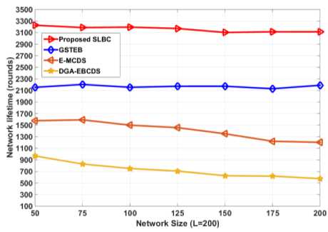
Fig.11. Comparison of network lifetime (First node dies)

• G.    Network lifetime with respect to percentage of dead nodes

As nodes have more remaining energy when the first node dies, this section analysis the network enhancement of algorithms until 30% of nodes are dead. Network size of this analysis is 200 nodes and the result shown in figure 12. According to figure 13, DGA-EBCDS unused maximum node’s energy, due to uneven energy distribution. Using this unused nodes energy, it shows improved performance in estimating the lifetime against the percentage of nodes death. After 30% of nodes dead, DGA-EBCDS prolongs network lifetime nearly 200% more than after the death of the first node. GSTEB prolongs the network lifetime more than 35% from its achievement when the first node dies. The algorithm E-

MCDS also increases the lifetime of network by 90% than its previous attainment. As, the proposed algorithm distributes nodes energy consumption evenly through energy aware node distribution (fitness based CH selection) and on-demand re-clustering method, the maximum node energy is used before the first node dies (as discussed in subsection V(E)). So, it prolongs the network lifetime by 26% from its own attainment. However, the proposed algorithm shows the network lifetime more than 22%, 55% and 76% compared to GSTEB, E-MCDS and DGA-EBCDS respectively, when the 30% of nodes are dead.

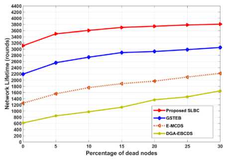
Fig.12. Comparison of network lifetime for percentage of dead nodes

• H.    Energy utilization of the nodes

Prolonging network lifetime through an efficient energy distribution among nodes is the primary objective of the proposed algorithm. When the algorithm succeeds in energy distribution, it utilizes more nodes energy to enhance the network lifetime. Nodes remaining energy at the end of each simulation is obtained and considered for the analysis of nodes energy utilization. The comparison of nodes average residual energy against network lifetime when the first node dies is shown in figure 13 and the comparison of energy utilization of nodes when the percentage of dead nodes is shown in figure 14. As DGA-EBCDS suffers heavily due to uneven energy depletion issue, CHs die prematurely. So, it leaves more network energy unused. E-MCDS also fails to distribute the nodes among cluster, so CHs from dense cluster die earlier, leaving maximum network energy unemployed. Also nodes in GSTEB experience more data forwarding, especially those nearer to the root. This leads to shorter network lifetime, leaving significant amount of network energy unemployed. But, the proposed algorithm, avoids CHs premature death through on-demand rotation scheme with negligible re-clustering overheads and reduces the nodes data transmission energy cost through proposed IND process. Then, nodes energy consumption is efficiently distributed over the network. So, the proposed SLBC algorithm employs more nodes energy and significantly prolongs the network lifetime. The proposed SLBC algorithm is uses the network energy nearly 20% more than the immediate performer GSTEB achieving 30% of lifetime enhancement. It also proves that the proposed algorithm consumes least amount of nodes energy than the compared algorithms for one round of data gathering. Figure 13 and 14 infer that the proposed algorithm efficiently utilized the node’s energy in order to enhance the network lifetime.

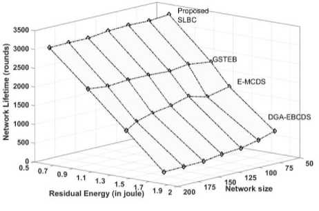
Fig.13. Comparison of energy utilization of nodes (first node dies)

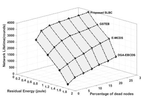
Fig.14. Comparison of energy utilization of nodes (when the percentage of dead nodes)

• VI. Conclusion

Efficient energy consumption of nodes is significant to prolong wireless sensor network lifetime, as it comprises power-constrained sensor nodes. In this paper, the algorithm SLBC is proposed to extend WSNs lifetime. SLBC extends WSNs lifetime by constructing the CDS with CHs being chosen based on a defined node’s weight. During CDS selection, nodes are evenly distributed among CHs, using an independent node distribution procedure. The proposed algorithm also evades control message overheads of re-clustering through an on-demand rotation scheme. Through an optimal CDS selection and even load distribution procedure, the proposed algorithm significantly prolongs network lifetime than the recent algorithms DGA-EBCDS, E-MCDS and GSTEB. Simulations results show that SLBC achieves network lifetime more than 30%, 55% and 200% compared to the recent algorithms GSTEB, E-MCDS and DGA-EBCDS respectively.