Sequential Adaptive RBF-Fuzzy Variable Structure Control Applied to Robotics Systems

Published Online August 2014 in MECS

Robust control structures are widely applied to control robot manipulators which are known to be highly coupled nonlinear systems [1].

Robots are usually exposed to load variations, uncertainties and disturbances which make them very hard to control. Variable structure controllers are robust schemes that use a high gain switching term to drive the system states toward a specific surface and maintain the system along it [2].

These controllers are robust against structured and unstructured uncertainties, but they have two important drawbacks:

The first one is high frequency oscillations in the control signal (chattering) and the other is the model dependency where the knowledge of the exact system parameters is required to compute the equivalent control. Several researches works have been developed over the use of neural networks and fuzzy techniques to fix up such disadvantages.

Authors of [3] used a fuzzy controller to compute the gain K in the discontinuous control part while [4] trained one RBF network to estimate the global robot model function. In [5], a sliding mode control with a neural network is used to predict the unknown interconnection terms of nonlinear interconnected systems. In [6], fuzzy sliding mode control is used to control nonlinear systems with structured and unstructured uncertainties with feedback linearization.

Authors of [7] trained one layer MLP neural network to design a sliding mode of single and coupled inverted pendulum. A neural adaptive based sliding mode controller is designed to trajectory tracking for mobile robots in [8].

Radial basis function (RBF) neural networks with their approximation capabilities [9] are very emergent powerful tools for system identification, so they can estimate any complex nonlinear system parameters even in presence of disturbances [10] [11].

In this paper, and to overcome the variable structure control lacks, a hybrid control law is proposed where four RBF networks are used to estimate the model parameters for the equivalent control taking advantage from the basic knowledge of the robot dynamic model. To eliminate the chattering, the corrective control part is designed with a fuzzy controller to update the gain so to avoid the use of a constant predefined value.

To train the proposed networks, a sequential training algorithm based on Growing-Pruning (GAP) strategy and Kalman filter is implemented [9]. A similar approach in [12] was applied to control two degrees of freedom robot manipulator where we ignored the frictions. The present work represents an extension of [12] where a fuzzy controller is implemented and neuron significance is introduced in the GAP criteria. The proposed approach is implemented to control a more complex nonlinear plant, three degrees of freedom RRP SCARA more constrained system than two degrees of freedom robot system used in [12] with consideration of frictions and disturbances.

The remainder of this paper is organized as follows:

Section 2 is dedicated to the variable structure controller while in section 3; the main steps of GAP-EKF are explained. The application of the fuzzy-RBF based variable structure control is presented in section 4. Simulations results are summarized in section 5. Section 6 gives some concluding remarks.

• II.    Variable Structure Control Scheme

• A.    The robot model

The dynamic equation of a manipulator of n degrees of freedom is given by (1) [2]:

M ( q ) q + C ( q , q ) q + G ( q ) + F ( q ) =Γ             (1)

where q , q , q are position, velocity and acceleration vectors respectively, Γ is the actuators torques vector. M(q) is the symmetric and positive definite inertia matrix, C ( q , q ) is the Coriolis/Centrifugal matrix while G(q) is the gravity vector. F ( q ) is the friction terms vector.

In the sequel, we will use the symbols M, C, G and F instead of M(q), C ( q , q ), G(q) and F ( q ) ).

• B.    Variable structure controller

A classical variable structure control is designed based on driving the robot states to slide over a surface s where all motion in neighborhood of the manifold is driven toward it [2][14].

Let's define the tracking error like:

e = q - q_d .                                        (2)

where q is the desired position and q is joint position. The sliding surface is defined by [14]:

s = e + λ e .                                       (3)

where λ = diag [ λ , λ  . λ ] , λ is a positive constant.

We have to choose λ so that the energy of the system will decay when s is not null, so it has to satisfy the condition [2]:

• 2 dt s≤-η sI .

The variable structure controller is given by:

Γ =Γeq +Γcc .

where the equivalent control part is given by:

Γeq = Mˆ (q)qr +Cˆ(q,q)qr +Gˆ(q)+Fˆ(q).

and the corrective one is defined by:

Γcc = -Ksign(s).(7)

Mˆ ,Cˆ,Gˆ,Fˆ are estimations of M ,C ,G and F respectively [2]. K=diag [K ,K   K ] is a diagonal positive definite matrix in which K is a positive constant and q is given by:

q_r = q_d - λ e , q_r = q_d - λ e .                     (8)

The closed loop relation is given by [2]:

Ms + Cs = ∆ f - Ksign ( s ).                      (9)

where Δ f  is the estimation error:

∆ f =( M ^ˆ - M ) q + ( C ^ˆ - C ) q + ( G ^ˆ - G ) + ( F ^ˆ - F ).

To prove the stability of the proposed controller, a positive definite Lyapunov function candidate V and its time derivative are given by [2]:

V (s)=  sTMs.(11)

V (s)= I ∆f -K I .(12)

The closed loop system is stable if the gain K is chosen greater than the boundary of uncertainties [2]:

K>∆f.

In a real environment, we have an imprecise idea about the value ∆ f and to ensure the stability of the controlled robot we have to work with high gains which cause high frequency oscillations and discontinuities in the control signal.

The designer has to estimate the exact model of the robot to minimize the boundary of ∆ f , and decrease the value of K to cancel the effect of chattering, which is not always evident due to disturbances, friction and uncertainties. This estimation could be done efficiently by using Radial Basis Function "RBF" with sequential training.

In other hand, the value of the gain K is estimated by a fuzzy controller so to start with high values when the states of the system are far from the surface and decrease the gain value near the sliding surface.

• III.    RBF Sequential Training Algorithm

• A.    RBF Network description

Radial basis function networks (RBF) are a variety of artificial neural networks[20]; they have one hidden layer and a linear output. The network output y ˆ =[ y ˆ₁, y ˆ₂,... y ˆ _Ny ] is given by (14) [10]:

y ˆ = f ( X )= Φ ^T ( X ) A .                         (14)

A =[a ,a ,  ,a ] is the weight's vector connecting the hidden layer to the output layer with N is the hidden layer neurons number, ΦT (X ) is the response of the hidden layer to the input vector X = [x ,x ,  ,xNx ] , Nx and Ny are the inputs and outputs dimensions respectively and Φ is the Gaussian function given by [9]:

X - µ I²

Φ ( X )=exp( - ).                      (15)

σ

µ is the center's vector of the hidden neurons and σ is the width of the Gaussian function.

• B.    Sequential network training algorithm

To obtain the desired behavior y responding to the input x , where i is the sample index, the neural network is trained using a sequential algorithm with a Growing and Pruning strategy (GAP) [9] to optimize the network architecture and an Extended Kalman Filter to adjust the network parameters. The growing of the RBF neural network is controlled regarding the neuron's influence in the global output [13]. The influence of the j th neuron is given by :

Inf j =	1.8 o N x ) aj	.                                (16)
	N Я1.8 - =1

• 1) . Growing criterium

While using and training the network, the algorithm decides to add a new neuron to the network if the criteria in (17) and (18) are satisfied [13]:

II x     M r\ |> S i .                                           ⁽¹⁷⁾

'      >  S . .                       (18)

Nx (1.8— j=1

where:

• e. = y.(xi)-yi(xi)

and

S = max { s у, s  }.(20)

i              maxmin

M_r are the centers of the closest hidden unit to current input x .

S S , S and у are thresholds to be selected , maxmin appropriately. Equation (17) checks if the current input data x are far from all existing hidden neurons so they can not reproduce the desired outputs while (18) checks if the influence of the new added N+1 node is greater then a threshold s . m

The parameters of the new added neuron are described in (21):

a N + 1 = e i

M n + 1 = x i

^ N + 1 = ^K||xi - M ir ||

where к is the overlap factor.

• 2) . Adjusting the network parameters with EKF

If the growing criteria in (17) and (18) are not met, only the network parameters of the nearest node to the current inputs are updated using the extended Kalman filter (EKF) as follows [9]:

w r = w r _{- 1} + Ke i .                              (22)

The vector w ^r contains the weights, centers and width of the nearest neuron to the current input data x :

w r = [ a . , и. , o _r ] .

and K is the Kalman gain matrix witch is computed for every new input/output data by:

K i = P - 1 B i [ R i + B l P i - 1 B i ] ^{- 1}.

B_f = 4, y is the gradient matrix of the function y .

R is the variance of the measurement noise. P is the error covariance matrix which is updated by:

P i =[I z . z - K i B T B i AP i - 1 + q 0 I z . z .                (25)

q is a scalar that determines the allowed random step in the direction of the gradient matrix. If the number of parameters to be adjusted is z , then P is a z x z positive definite symmetric matrix. When a new hidden neuron is added, the dimensions of P will be:

p = | P ^{- 1}

¹ I 0

q 0 I g . g

The new rows and columns are initialized by q (an initial uncertainty estimation). g is the number of new parameters introduced by the new hidden neuron.

• 3) . Pruning criterium

For each presented data, the j ^th neuron could be deleted if the criterium in (27) is verified:

(1.8 ^ -) ^Nx

N 1 ( 1.8 ^ -) Nx j =1

where e is a pruning threshold to be selected.

• IV.    RBF-fuzzy Based Variable Structure Controller

• A.    RBF Network based equivalent control

To fix the problems of model dependency of the variable structure controller in (5), four RBF networks are trained online to estimate the parameters of matrices M , C , G and F in (6).

The main idea is to use RBF networks defined in section III to estimate the parameters of the equivalent control. The networks are online trained using the GAP-EKF based algorithm. In this work we use a RBF network to estimate inertia matrix M, another one to estimate Coriolis matrix C, a third RBF neural network to estimate gravity vector G and the last one is used to compensate friction terms F . The outputs of the RBF networks are the estimated components of the model matrices as given in (28, 29, 30 31)

M ^ˆ ( q )= f M ( X M )

= ® L ( X m ) A m , X m =[ q T ]

C ^ˆ( q , q )= f C ( X C )

= Θ ^T C ( X C ) A C , X C = [ q^T , q^T ]

G ^ˆ( q )= f G ( X G )

= Θ ^T G ( X G ) A G , X G =[ q^T ].

F ^ˆ( q )= f F ( X F )

= Θ ^T F ( X F ) A F , X F = [ q^T ].

where θ = [ θ ¹,..., θ ^m , θ ^M ] ^T is the y membership functions                 centers                 vector.

ϖ ( x ) = [ ϖ ¹( x ),..., ϖ ^m ( x ), ϖ ^M ( x )] ^T is the vetcor of heights of the output y membership functions and ϖ ^m ( x )is given by[21]:

ϖ ^m ( x ) =

∏ ⁿ µ _A m ( x_i ^*)

= i

M

∑∏ _i ⁿ _{= 1} µ A im ( x i ^*)

m = 1

where f ,f ,f and f are four independent RBF neural networks with inputs X ,X ,X   and X .

MCG   F

Their weights vectors are A ,A ,A and A MCG    F respectively

Equation (6) becomes:

Γ eq = Θ ^T M ( q^T ) A M q r +Θ ^T C ( q^T , q^T ) A C q r + Θ ^T G ( q^T ) A G +Θ ^T F ( q^T ) A F .

The resulted RBF based equivalent control is shown in Fig.1.

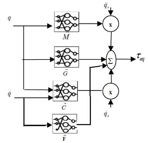
Fig 1. RBF based equivalent controller

• B.    Fuzzy corrective control

Usually, a fuzzy system has one or more inputs and a single output with a rule base and an inference engine as showed in Fig.2. The rules in the rule base are in the following form [15]:

IF xi is Ai THEN yi is Bi where Ai and Bi are fuzzy sets

The output of the fuzzy controller is given by (33) [16]:

M

∑ θ ^m ∏ _i ⁿ _{= 1} µ A_i m ( x i ^* )

y = ^{m =} _M ¹                  = θ ^T ϖ ( x )               (33)

∑∏ _i ⁿ _{= 1} µ A im ( x i ^* )

m = 1

where M is the amount of rules

The corrective control in (7) is obtained by a fuzzy controller. The tuning rule for the gain K is to decrease its value near the sliding surface in order to damp the chattering amplitude and to increase it far from the surface. In this regard, a fuzzy controller rule base is proposed for tuning K as illustrated in table (1), in which inputs are the surface s and it’s time derivative respectively. (ZE: Zero; B: Big; M: Medium; N: Negative; P: Positive). For multiple-output system, they can be considered as a combination of several single-output systems.

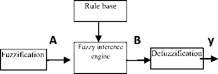
Fig. 2. Fuzzy controller

Table.1. Fuzzy rule base for tuning the gain “K”

s s	NB	NS	ZE	PS	PB
N	KB	KB	KM	KS	KB
Z	KB	KM	KS	KM	KB
P	KB	KS	KM	KB	KB

To design the corrective control, membership functions for the fuzzy controller input (surface s, its derivation) and the output (gain K) are presented in Fig.3, Fig.4 and Fig. 5.

The whole fuzzy-GAP-RBF neural networks based variable structure controller is shown in Fig.6.

• V.    Simulation Results

Simulations were carried out over a three dof RRP SCARA robot manipulator whose dynamic model is given by (35) [4]:

M ( q ) q + C ( q , q ) q + G ( q ) + F ( q )= Γ .           (35)

with:

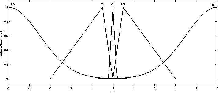
Fig. 3. Membership function of s (input 1)

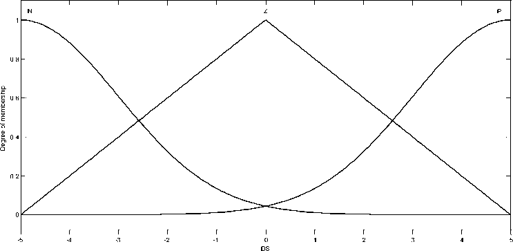
Fig. 4. Membership function of (input 2)

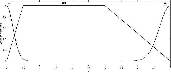
Fig.5. Membership function of K (output)

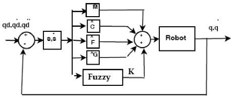
Fig. 6. Neural adaptive-Fuzzy variable structure controller

M_x , =2.1240 + 1.44 c os ( q_T )

M,₂ = - 0.4907 - 0.72 c os ( q ₂)

M =0

M ( q ) = ^ M ₂j = - 0.4907 - 0.72 cos ( q ₂)

M₂₂ = - 0.4907, M ₂₃=0

M = M = M =0

Г d

' C 1, = ^1.44q2sin(q 2 ) C₁₂ = - 0.72 q₂ .sin (q^ )

C (q , q ) = «	C 2 2 = - 0.72q2 .sin (q2 )
	C 13 = C 21 = C 23 = 0

c

= C = C =0

5 sin (2 t )

5 sin (2 t )

5 sin (2 t )

	Gx =0
	G =0
G ( q )=	2
	G з = - 4.9

F = 12q_x + 0.02 sign (q_x ) +

F (q ) = ^

3 sin (3 t )

F₂ = 12q₂ + 0.02 sign (q₂ ) +

3 sin (3 t )

F₃ = 12 q ₃ + 0.02 sign (q₃ ) +

3 sin (3 t )

We used the variable structure controller in (5) to control the SCARA robot where the Inertia, Centrifugal and Coriolis and friction model matrices are estimated using the proposed sequential algorithm. In our case (38), the gravity vector G ( q ) remains constant and does not need to be estimated.

(38)      To test the robustness of the proposed controller; we considered the disturbances in (40) and altered the parameters of the inertia matrix by adding a quantity km2 = 0.001 kg to the second link mass m2.

The desired trajectory to be tracked is a sinusoidal signal as shown in (41):

q_d =1 + sin ( n t )                                 (41)

The external disturbances are:

(39)      Fig.7, Fig.8, Fig.9 show the desired and real positions of the three joints and Fig.10, Fig.11, Fig.12 show the tracking error of the robot joints while velocity errors are presented in Fig.13, Fig.14, Fig.15. We see that both position and velocity errors are acceptable and converge toward zero in a short time (after 1s). That means that the proposed RBF neural networks (with the sequential learning algorithm) needed just few data samples to learn the robot behavior.

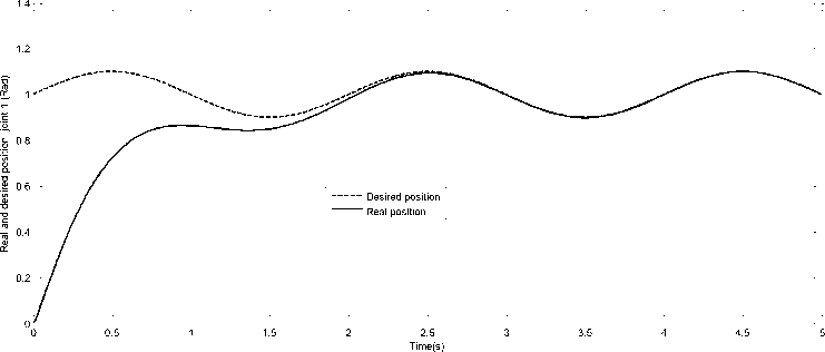
Fig. 7. Desired and real position of Joint 1

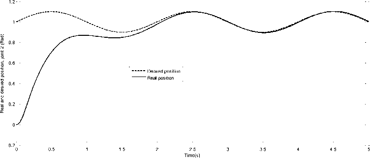
Fig. 8. Desired and real position of Joint 2

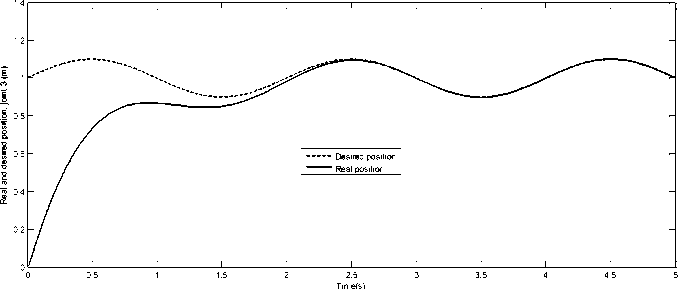
Fig. 9. Desired and real position of Joint 3

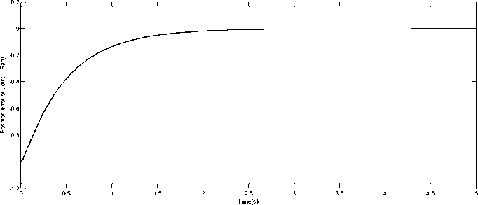
Fig.10. Position error of Joint 1

Position error of Joint 3(m)                                                                  Position error of Joint 2(Rad)

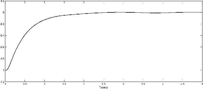
Fig.11. Position error of Joint 2

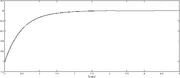
Fig. 12. Position error of Joint 3

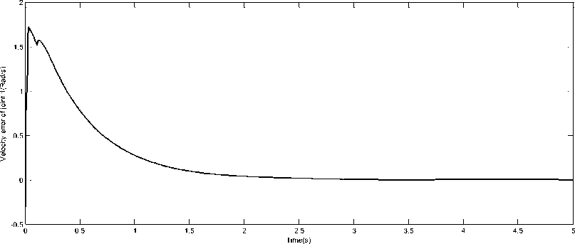
Fig. 13. Velocity error of Joint 1

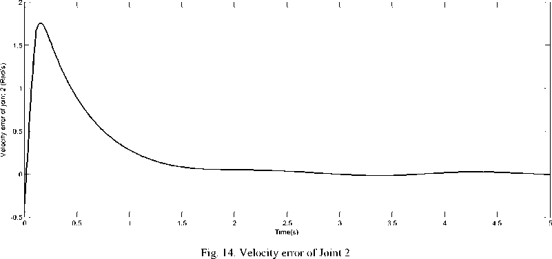
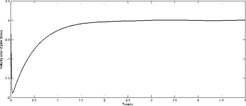
Fig. 15. Velocity error of Joint 3

Torques acting on the robots joints and sliding surface are presented in Fig.16, Fig.17, Fig.18 and Fig.19 respectively. We see clearly from the control signal figures that chattering is completely eliminated due to the good estimation of the model parameters and so we do not need to work with high gain values to compensate the model variations, uncertainties and external disturbances.

Values of the gain K are presented in Fig. 20 and we see that K is big far from the surface and when the system states are close to the sliding surface the values of k are decreased to be null.

Time(s)

Fig. 16. Control torque for joint 1

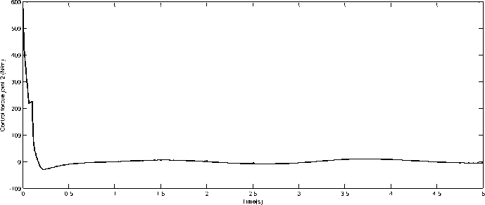
Fig. 17. Control torque for joint 2

^{liding surface}                                                                          Control torque joint 3 (N/m)

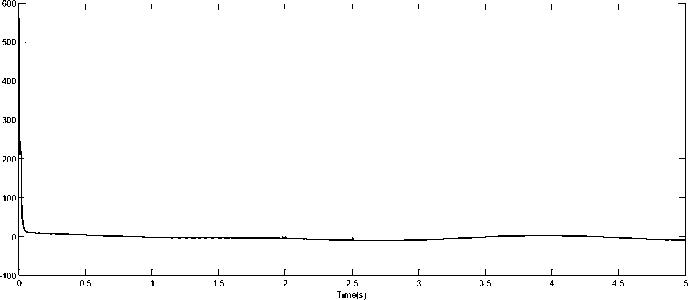
Fig. 18. Control torque for joint 3

Time(s)

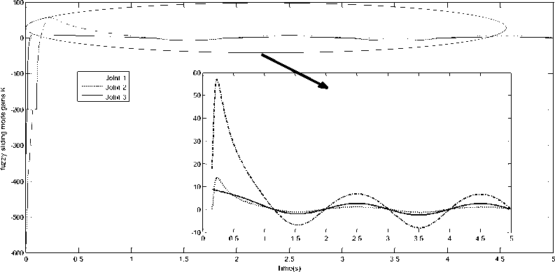
Fig. 20. fuzzy controller output (Gain K)

The training of RBF neural networks is achieved online during the control process. Table.2 summarizes mean square errors of training for the three RBF neural networks for each second of the simulation time (5s) in presence of external disturbances and model uncertainties.

Table 2. Estimation errors of the RBF neural networks

Seco-ndes	without disturbances and uncertainties			without disturbances and uncertainties
	M	C	F	M	C	F
1	5.41e-6	4.53e-8	1.16e-16	2.62e-5	9.21e-8	3.88e-15
2	6.27e-8	4.45e-8	2.22e-17	3.54e-7	6.55e-8	3.29e-16
3	2.49e-8	7.92e-8	8.88e-17	4.02e-7	8.22e-8	1.24e-16
4	1.56e-8	3.33e-8	3.05e-17	8.23e-7	5.36e-8	5.86e-16
5	2.85e-8	9.74e-8	8.72e-17	5.14e-7	1.94e-7	2.11e-16

The training errors are less then 1e -6, 1e-8, 1e -16 for estimating inertia, Coriolis and friction matrices respectively. These small training errors are due to the strength of the sequential training algorithm. Indeed, the fact that the training is achieved online, allows the RBF to react against any disturbance or model variation.

• VI.    Conclusion

We presented in this paper a variable structure controller for robot manipulator where the equivalent control was achieved using four radial basis function neural networks to estimate the robot matrices (Inertia,Centrifugal and Coriolis, Gravity and Friction). To enhance the estimation abilities of the networks, we implemented a sequential training algorithm to identify the model parameters online. The corrective control was replaced by a fuzzy controller to compute the K gain values along the control process.

The obtained results are very acceptable even in presence of uncertainties and the chattering problem of variable structure controllers is avoided.