Several cancer classifiers combined with PLS-DR for base on gene expression profile

Author: JianGeng Li, Hui Li
Journal: International Journal of Information Technology and Computer Science(IJITCS) @ijitcs
Article in issue: 4 Vol. 3, 2011.
Free access
It is known that Logistic Regression coupled with Partial Least Squares dimension reduction (PLSDR-LD) is capable of extracting a great deal of useful information for classification from gene expression profile and getting a rather high classification accuracy rate. In this study, we replace the logistic function of Logistic Regression with several functions which are similar to logistic function in appearance, and apply these functions to the analysis of microarray data sets from two cancer gene expression studies. We compare these newly introduced models with PLSDR-LD proposed in the literature. The most effective models with good prediction precision are lastly provided through analyzing the results of two experiments.
Logistic Regression, Partial Least Squares, gene expression profile, PLSDR-LD
Short address: https://sciup.org/15011628
IDR: 15011628
Text of the scientific article Several cancer classifiers combined with PLS-DR for base on gene expression profile
A vast amount of data generated through gene microarray, gives us sufficient biological information. Meanwhile, it brings us great difficulties to manage, integrate and interpret these data sets. Comprehensive approaches are needed to take full advantage of the huge information offered by the data. As a generally used statistical modelling method, PLS is first used in econometric path modeling by Herman Wold and afterwards it is used in chemometric and spectrometric modeling as a multivariate regression too[11-13]. Nguyen and Rocke proposed using PLSDR(PLS based dimension reduction) for dimension reduction as a preliminary step of classification, based either on linear logistic discrimination, linear or quadratic discriminant[9-10]. What attracts our attention is the classification method namely logistic discrimination. LD performs well in classification and has its own specialty when dealing with dummy variable. In this article, the application of sigmoid function to classification attains even better effect and a contrast with other like-logistic model will be given in the METHODS section. In recent years, many researches on PLSDR have been carried on embracing a great many aspects in various domains[7-8], besides, comparison have been conducted in the dimension reduction and discrimination realm[2]. The results of many experiments carried in the paper mentioned above demonstrate that PLSDR is an effective technique for dimension reduction. So PLSDR will be adopted in this paper, and the classical algorithm PCA is given to make a compare. Considering the fact that PLSDR is good at correlation but weak at remove irrelevant features among a set of complex features[14]. It is necessary to combine eliminating noise(irrelevant features) and dimension reduction into the ultimate model. As a result, we propose a model begin with irrelevant genes elimination. When the preliminary gene selection is finished, the process of dimension reduction (PLSDR and PCA) and classification are immediately implemented. These models would be used to dispose gene data sets. Some like-logistic functions are used in discrimination and the relevant results of classification are given in the Experiment part. In order to make a comprehensive comparison with logistic function, similar data processing method are adopted as Nguyen et al 2002b. The relevant indicators such as number of misclassification will be given in order to measure their swords in handling with biological information. Four data sets are used in the Experiment section in order to provide a stable result.
-
II. METHODS
A Gene Selection
The original gene data is rich of various kinds of biological information, but only a number of genes are of interest in our experiment. Of course, other genes are not of no use. They are just ‘misplaced resources’ and may play an important role in other practice. In every special experiment, the ‘noise’ may refer to different genes. So the elimination of irrelevant genes is necessary to improve the accuracy of classification and cut down on the calculation time spent on classification. Although the computing capacity of computer continues to expand, reducing the high computing complexity is of great significance because of the enormous volume of gene data sets. So in this article we employ the t-statistic scores to select the important genes. In this article, we just consider of binary classification problem. So the samples belong to two classes and the t-statistic score is given as:
x 0 — X 1
^var( x 0 )/ N 0 + var( x 1 )/ N 1
x 0 , x 1 is the mean expression value of two classes for a single gene. var( x 0 ) and var( x 1 ) are the variance respectively. N , N is the size of each class. Obviously, the bigger t-statistic score represents the more different expression in the two classes for a single gene. It could mean that a single gene behaves disorder in one type of the sample. So we could suspect that this gene is somehow related to the classification of samples.
B Some Classification Function
We find that some functions which like logistic can be used in classification problems. All of them are strictly monotonically increasing and invertible. The domains of those functions are all specified in ( -^ , +^ ) , the value domains are in [ — 1, + 1] .
In this paper, three logistic-like functions will be applied to the model of classification. The functional form are denoted in (3)~(5).
uk ( x )
uk ( x )
- e
|
f ( XX ) 2( e U t ( X ) + e" U t ( X ) ) 1 2 |
(3) |
|
|
f ( X ) = |
11 — argtan( uk ( x )) + - n z u k ( x ) t 1 e 2 dt n -^ |
(4) |
|
f ( X ) = |
(5) |
|
to corresponding category by comparison to the mean of n ( k | X ) of each sample. For example, k=1 denotes normal, k=0 denotes cancer. If the value of a sample n ( k | X ) is larger than the mean, the sample should be classified as normal, else as cancer.
Owing to the same principle behind classification method and the lack of space, the detail of Arg discriminate(AD) and Gausian discriminate(GD) are not given in this section.
D PLSDR and PCA
Here we give the process of the algorithm PLSDR,
1) Standardize the data,
The first one is a transformation of sigmoid function which is often used BP neural network. The second one is also a like-logistic function which is named Arg function for convenience. The last one is Gaussian Error function. The discriminate methods employing these three functions are expressed as SD AD and GD respectively in this paper.
~ x ij
X ij -
s j
x j (i=1,2,….n; j=1,2,……p)
C
Sigmoid Discriminate
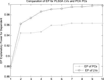
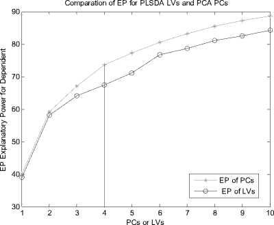
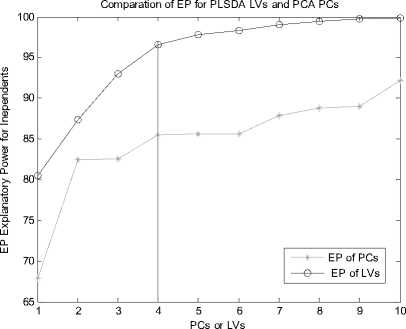
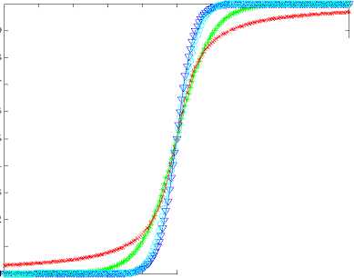
Let X is the gene expression data set. Before all the treatment on this set, it should be centered to zero mean. The original data X is n*p(i=1,2,3…,n; j=1,2,3…,p), the column of X represents the microarray sample of data, the row represent the expression level for each gene. After preliminary gene screening and dimension reduction, the number of columns of independent variable namely X has reduced from p to k(k If we use linear probability model to simulate the relationship between X and Y, encountering lots of problems will be inevitable. Firstly, y should not be limited in a range of values, because independent variable X, regression coefficients and residuals are preferable of an arbitrary value. However, in our experiments, y is dummy variables. Secondly, there is different variance for different observations. It is contrary to Gauss - Markov assumption. This is called hereroscedasticity. Thirdly, the relationship between observations and variables is mostly likely nonlinear[3]. So in this section, we introduce a new kind of model which is inspired by logistic regression[7]. In sigmoid regression, the condition class probability, П = P(y=1|x) = P(sample is classified to tumor for gene profile x) is modeled using the sigmoid functional form. Sigmoid function is usually used in BP network. It is denoted as: n(k | x) = ep.»+x,iP,i+x 2 Pi2+... xpPp eP« + Xi1Pi1 + xi2Pi2 +~ XipPip + e ke {0,1} Uk (X) = вп + X.в1 + X ?A? + ...X. в k i0i1i1i2i2 ipip conditional class probability is . So the ultimate ~ yi sy (i=1,2,…n) xj is the mean of xj , sj is the standard deviation ofxj , y is the mean of yi , sy is the standard deviation of yi .We use E0 to denote the standardized form of X, F0denotes Y. 2) We extract the first component u1from F0, u1= F0c1, c1=1. And we extract the first component t1from E0, w1=1. In binary classification, u1= F0, so, EoFo =(E1, Ев,..., Ep )F =(r(x, y) r(x2, y),..., Кxp, y))' (6) w = r(x1,y) r(x2 ,y). p Zr2(xj, у) ... r(xp, y) t1= E0w1 I p1 [r(^,y)E01 +r(X2,y)E02 +".+r(Xp,y)E0P]( Zr2(xj’ y) 3) We can get the residual matrix Eh and Fh , euk(x) n(k | x) =------- 2(euk(x) e - uk( x ) । e uk(x) I )2 ke {0,1} Estimate of p is obtained by maximum likelihood estimation(MLE). The estimated value is denoted as pE . With this value, a given sample can be endowed with a sigmoid probability value. With this value the sample can be classified F = F -t n ’ = F -t h-1 h Eh Eh-1 thph Eh-1 th n M2 th F = F -t r ’ = F -t h-1 h 1 h 1 h-1 thrh 1 h -1 th ц m2 th2 4) We use Eh to replace E0, Fh to replace F0. Repeat the second step. Lastly, we get all th and uh . The process of PCA is given, 1) Standardize the data, xij xj xij = (i=1,2,….n; j=1,2,……p) (11) sj xj is the mean of xj , sj is the standard deviation ofxj . 2) Calculate the correlation matrix R (p*p) of X. 3) Calculate the eigenvalues λ1≥λ2≥... ≥λh ,and the relevant eigenvectors a1, a2,..., ah . 4) Get the hth principal component, p Fh=Xah=∑ahjxj (12) j=1 ahj is the jth component of ah . III. EXPERIMENTS A Acute leukemia data Gloub et al.(1999) published the acute leukemia data set, which is widely used. The original data set consisted of 47 Acute Lymphoblastic Leukemia(ALL) and 25 Acute Myeloid Leukemia(AML). It consisted of 62 bone marrow samples(from adult patients) and 10 peripheral blood specimens(from adults and children) containing probes for 7129 genes. At first, gene selection comes on stage. After that, PCA or PLSDR is used to decrease the dimension. In every step of PCA and PLSDR iteration, there is an residual. The explanatory power(EP) of principal components and latent variables can be represented by ratio of residual and dependent variable. Figure1 and Figure2 give the EP for predictor variables and response variables of the top 10 LVs and PCs. From Figure 1, we can conclude that PCA performs better than PLSDR in interpreting response variables. The top ten of PCs can stand for 95.96% of predictor variables while PLSDR is 94.91%. They give the similar results in interpreting the predictor variables. However, the PCA gives a much worse performance in EP for dependent variable. Note that the EP values bounces around the fourth PC and then goes steady. This is typical of PCA because the factors are not determined with regard to response variables. So the sharp difference between PLSDR and PCA in Figure 2 is beyond doubt. From Figure 1 and Figure 2, we can also conclude that the number of PCs or LVs(latent variables) in Nguyen et al[10] make sence. The explanatory power for independent variable increase less than 2% when putting the 4th LV into consideration. Meanwhile, we S get the value of , through SIMCA-P, it is 0.9425 > SSS,3 Fig. 1 Explanatory Power for Independent Variable of PLSDR and PCA PCs or LVs Fig. 2 Explanatory Power for Dependent Variable for PLSDR and PCA We divide the original data set into two parts. One is used as training samples(38 samples, 27 ALL, 11 AML), while the remaining are used as test samples(34 samples, 20 ALL, 14 AML). For the training data, we use leave-one-out CrossValidation to assess the fitness of LD SD AD and GD. All methods predicted the ALL/AML class correcly 100% for the 38 training samples with all these discriminate methods. The test data set are used to evaluate the performance of models and which provides additional protection against overfitting. One of the AML samples (#66) is classified into ALL incorrectly by LD SD AD and GD, which is also misclassified by Golub et al 1999 using a weighted voting scheme. In table 2, SD and GD give an equivalent performance in the discrimination procedure. When P*=500 and P*=1000, SD and GD get the best result among the four methods. AD’s classification ability is relatively weaker than the other three methods. It makes another error in the test data set (#42) besides the sample #66 based on P*=50. Table 1. ALL-AML data classification results of LD SD AD and GD(pca). Given are the number of samples correctly classified in the 38 training set and 34 test set. P* Training data Test data (leave-out-one CV) (out-of-sample) LD1 SD AD GD LD SD AD GD 50 38 38 38 38 33 33 31 33 100 38 38 38 38 32 32 30 32 500 38 38 38 38 31 31 30 31 1000 38 38 38 38 31 31 30 31 1500 38 38 38 38 30 31 29 31 Table 2. ALL-AML data classification results of LD SD AD and GD(pls). Given are the number of samples correctly classified in the 38 training set and 34 test set. P* Training data Test data (leave-out-one CV) (out-of-sample) LD SD AD GD LD SD AD GD 50 38 38 38 38 33 33 32 33 100 38 38 38 38 32 33 31 33 500 38 38 38 38 31 33 30 33 1000 38 38 38 38 31 31 30 31 1500 38 38 38 38 31 31 29 31 Table 3. ALL-AML data re-randomization(36/36 spliting) classification results of LD SD AD and GD(pca). Given are the correct classification percentage averaged over 100 rerandomizations. P* Training data Test data (leave-out-one CV) (out-of-sample) LD SD AD GD LD SD AD GD 50 34.08 34.05 33.53 34.10 33.66 33.61 33.15 33.59 100 33.29 33.44 32.96 33.39 32.92 34.06 32.43 34.12 500 34.32 34.13 34.17 34.12 34.08 33.97 33.74 33.91 1000 32.95 33.19 33.02 33.17 32.50 32.78 32.62 32.81 1500 32.51 32.65 31.98 32.77 32.11 32.21 31.29 32.24 Table 4. ALL-AML data re-randomization(36/36 spliting) classification results of LD SD AD and GD(pls). Given are the correct classification percentage averaged over 100 rerandomizations. P* Training data Test data (leave-out-one CV) (out-of-sample) LD SD AD GD LD SD AD GD 50 36.00 36.00 36.00 36.00 34.72 35.11 34.83 35.10 100 35.88 36.00 35.82 36.00 34.30 34.71 34.32 34.68 500 36.00 36.00 36.00 36.00 34.73 34.68 34.28 34.73 1000 36.00 35.98 35.97 35.98 34.82 34.85 34.61 34.86 1500 36.00 36.00 35.97 36.00 34.71 34.77 34.50 34.78 The number of samples correctly classified by LD is from Nguyen 2002b[10]. The re-randomization study is also carried out on the Leukemia data set to assess the stability of the results shown in Table 1, 2 and make a good compare among the four discrimination methods. The 72 samples are equally random divided in two parts: N1=36 training and N2=36 test samples. This analysis is also repeated for 100 re-randomizations for the purpose of utilizing the result of Nguyen et al. 2002b[10]. The results in the column of Table 4 are better than the corresponding value in Table 3. Careful study of each line of test data in Table 4 showed that the effectiveness of SD as well as GD is the same or even better than LD. AD give a worse performance than the other three discriminating methods. Analyzing the corresponding row of Table 3 and Table 4, we can get that PLS definitely give a perfect result in dimension reduction, whereas, PCA is slightly worse. Table 5. Colon data classification results of LD SD AD and GD. Given are the number of samples correctly classified out of the 62 samples(40 tumor 22 normal). P* LD SD AD GD PC PLS PC PLS PC PLS PC PLS 50 54 58 55 59 53 58 55 59 100 53 58 54 58 53 56 54 58 500 53 56 53 56 52 54 53 56 1000 52 57 54 56 51 55 54 56 B Colon data Alon et al.(1999)[1] used Affymetrix oligonucleotide arrays to monitor expression of over 6500 human genes with samples of 40 tumor and 22 normal colon tissues. Alon et al. clustered the 62 samples into two clusters. One cluster consisterd of 35 tumor and 3 normal samples(n8, n12, n34). The second cluster contained 19 normal and 5 tumor tissues(T2, T30, T33, T36, T37). Furey et al.[5] did leave-out-one CV prediction of the 62 samples using SVM and six tissues are misclassified, namely(T30, T33, T36) and (n8, n34, n36)[10]. Note form Table 5, SD and GD give the best performacne in classification. The two samples T36 and n36 are correctly classified into the relevant category (with conditional class probabilities 0.89 and 0.12). Because SD and GD are not based on the same proposed hypothesis as describled in T.S Furey et al.(2000). However, the SD and GD misclassify the same samples (T2, T11, T33 ) as SVM and cluster. The ‘Prediction Strength(PS)’(Golub et al.1999) of these samples are all low(PS<0.30). Three tumor samples are classified to normal class by all four discrimination methods. SD and GD do not make mistake as LD and AD on sample n36. Besides, the SD and GD give a similar result considering the conditional probability, and the result is slightly better than the other two methods in discrimination. From Figure 3, we can also get that SD and GD conditional probability for tumor samples are all closer to 1 and the value for normal samples are all closer to 0 than the other two. The misclassified samples are marked on the horizonal axis. Almost all the small circle and triangle are above the blue star in the tumor part, and below the blue star in the normal part. Conditional Probability of LD SD AD and GD 0.9 I ^ 0.8 LD SD AD GD 0.7 0.6 0.5 0.4 0.3 0.2 Г v 0.1 T11 T33 n... n36 0 1ш T2 sample sequence Fig. 3 Conditional Probability of LD SD AD and GD based on p*=50. Misclassified samples are labeled on horizontal axis. Why PCA fails to make a prediction for response variable. The answer can be found in Table 6. Note that four components extracted by PLS base on 50 pre-selected genes can explain 95.00% and 91.16% of predictor and response variability respectively while the variability explained by the components of PCA are 95.46% and 76.45%. PLS and PCA give a similar performance in explaining the variation of predictor. Table 6. Variability explained by PLS components and PCs. The number of components base on 50 pre-selected genes is K. K Predictor Response Proportion Cumulative Proportion Proportion Cumulative Proportion PLS 1 81.43 81.43 83.22 83.22 2 7.42 88.85 3.89 86.11 3 5.39 94.24 2.04 88.15 4 0.76 95.00 2.01 91.16 PC 1 81.52 81.52 73.12 73.12 2 11.53 93.05 1.05 74.17 3 1.43 94.48 0.03 74.40 4 0.98 95.46 2.05 76.45 But PCA interprete only 76.45% of response variability which is much poorer than PLS. The second component of PCA accounts for predictor variablity is 11.53% but it accounts for only 1.05% of total response variability. The theoretical reason can be found in section 2.4. Due to these analysis, PCA fail to make a precise prediction as well as PLS is not surprising. Table 7. Lymphoma data classification results of LD SD AD and GD. Given are the number of samples correctly classified out of the 74 samples. P* LD SD AD GD PC PLS PC PLS PC PLS PC PLS 50 72 73 72 72 72 71 72 72 100 72 71 72 71 72 71 72 71 500 72 71 72 71 71 70 72 71 1000 72 70 72 71 71 70 72 71 Table 8. Lymphoma data re-randomization(37/37 spliting ) classification results of LD SD AD and GD(pca). Given are the correct classification percentage averaged over 100 rerandomizations. P* Training data Test data (leave-out-one CV) (out-of-sample) LD SD AD GD LD SD AD GD 50 36.3 1 36.02 35.86 36.02 36.12 35.85 35.15 35.85 100 36.36 36.41 36.18 36.41 36.26 36.23 35.43 36.21 500 35.23 35.39 35.02 35.42 35.31 35.42 34.74 35.42 1000 34.98 35.11 34.90 35.11 33.94 34.01 33.42 34.01 Table 9. Lymphoma data re-randomization(37/37 spliting) classification results of LD SD AD and GD(pls). Given are the correct classification percentage averaged over 100 rerandomizations. P* Training data (leave-out-one CV) Test data (out-of-sample) LD SD AD GD LD SD AD GD 50 36.92 36.91 36.48 36.91 35.57 35.63 34.83 35.63 100 36.91 36.95 36.51 36.94 35.84 36.02 34.92 36.02 500 36.86 36.85 36.22 36.85 35.76 35.93 34.88 35.93 1000 36.84 36.88 36.08 36.88 35.61 35.49 34.61 35.49 C Lymphoma data The data set presented by Alizadeh et al. (2000) comprises the expression levels of 4151 genes from 3 different classes: Diffuse Large B-Cell lymphoma (DLBCLL; n1=45), B-Cell Lymphocytic Leukemia (BCLL; n2=29) Follicular(FL; n3=9). In order to test our binary classification method and make a compare with logistic discrimination[10]. We chose the first two class, namely DLBCLL and BCLL. We got the value of PRESS,4 SS,3 using SIMCA-P, it is 0.8579 < 0.9025. So the 4th LV should be considered in the subsequent process. Lastly, using LOOCV, each sample is predicted to be DLBCLL or BCLL base on 5 gene components constructed from p*=50,100,500,1000 genes. The two samples(#33 and #51) are consistently misclassified. Table 7 and Table8 provide the detailed consequence of LD SD AD and GD. All these methods can be used as means to predict the samples, because they achieve perfect result in the procedure. As with the analysis of acute leukemia data, we turned to re-randomization to access the stability of the classification performance. Table 8 and Table 9 are the results using PCA and PLS to reduce dimention respectively. Compare with Table 7 in Nguyen 2002b[10], the accuracy rate of classification base on 5 components is impoved appreciably. All the classification methods displayed rather good ability in discrimination. Especially the LD SD GD, the accuracy rate for training data using LOOCV is nearly 100%. The accuracy is best for p*=50, which denoted that gene select process is of great importance for the entire experiment. Because this process filtered the irrelevant gene which may be interference to the prediction procedure. D Gastric cancer data This gastric cancer data contains the probes of over 19900 human genes with samples of diffused ones and intestinal ones(20 diffused and 20 intestinal). All the samples which are microarray data base on specimen of gastric carcinoma and clinical data are from China. They are all supplied by Beijing Cancer Hospital. In this experiment, we employ similar procedure with the above practice to deal with the original data set. The EP is vary for different preliminary selected gene number. We use the mean of EP which is calculated from each row of Table 2 for the purpose of ruling out of chance. In these two Figures(Figure 4 and Figure 5), a vertical line is drawn at number of LVs or PCs equals 4. The fifth LV can just interpret 1.24% of response variability, so we use top 4 LVs in the classification process because the 5th LV is of little use(less than 2%). This method is proved to be as effective as S ,in the following experiment. The advantage of SSS,i-1 PLSDR in interpreting response variablity is much more obvious than PCA. Correspondingly, the classification accuracy is much better for PLSDR than PCA. In order to further certify the effectiveness of LD SD AD and GD. We compare the four models using this data set. The result is exhibited in Table 10. The difference in explaining the response variability of PCA and PLS makes an interpretation for the gap of classifiction results. The number of misclassified samples is the same for LD SD and GD base on P* = 50, however the samples are disparate. (#11, #18)for LD,(#11, #24)for SD(#11,#18) and GD(#11, #24). AD gives the worst performance no matter how many genes are considered. The rerandomization is no longer provided, because the number of sample is too small. Fig. 4 Explanatory Power for Predictor Variable of PLSDR and PCA Note from Table 5 that with the decrease of gene number, the classification accuracy is increasing. It proves that gene selection is of a significant role in this experiment. IV. ANALYSE AND CONCLUTION Why SD and GD are competitive or even better than LD, AD gives the worst performance. Here we give the compare of these function curves in Figure 6. From it, we can see that there is no distinguishment between them in the outline of curve. However, we should pay attention to the sharp boosting of sigmoid function. The sharpness gives the opportunity of less iteration in the algorithm of determining the coefficient. As a result, it achieves better results in saving time of step-by-step process. The Logistic function curve overlaps with Gaussian Error function. So they give a similar result in classification procedure. Fig. 5 Explanatory Power for Response Variable of PLSDR and PCA Table 10. Gastric cancer data classification results of LD SD AD and GD. Given are the numbers of samples correctly classified out of the 40 samples. P* LD SD AD GD PC PLS PC PLS PC PLS PC PLS 50 35 38 35 38 35 38 35 38 100 35 38 35 38 35 37 35 38 500 34 38 34 38 33 37 34 38 1000 34 37 35 37 33 36 35 37 2000 34 37 34 37 33 36 34 37 Logistic Sigmoid Argtan fun and Gaussian Error 0.9 0.8 0.7 0.6 0.5 0.4 0.3 0.2 0.1 -8 -6 -4 -2 0 2 4 6 8 10 Logistic function Sigmoid function Argtan function Gaussian Error value of x Fig. 6 Comparison of Logistic function and Transformed Sigmoid function The value domain of red curve is a smaller range than the other three functions in Figure 6, which is the reason of poor discrimination ability of AD. In Figure 3, the effectiveness of SD LD AD and GD has been already obtained from one side. And the result is agreed with which concluded from the figure above. This article gives comparative study of some new models to classify samples base on microarray dataset. The tool presented here can achieve better or competitive result compare with PLS-LD (PLS-Logistic Discriminate). Our experimental codes which programmed by MATLAB language are all carried out on a PC workstation with Intel Core DuoT2060 (1.6G) and 4GB RAM. Acknowledgement Thanks Professor Lu Youyong from Beijing Cancer Hospital for providing gastric cancer data to us. This research is Supported by Beijing Natural Science Foundation (Grant No.4092021) and Scientific Plan of Beijing Municipal Commission of Education (JC002011200903). V. REFERANCE [1] Alon, U. Barkai,N. Notterman,D.A. Gish,K. Ybar,S. Mack,D. and Levine,A.J. Broad patterns of gene expression revealed by clustering analysis of tumor and normal colon tissues probed by oligonucleotide arrays. Proc. Natl Acad. Sci. USA,1999;96,6745-6750. [2] Boulesteix,A.-L. PLS dimension reduction for classification of microarray data. Statistical Applications in Genetics and Molecular Biology. 2004;3(1),33. [3] Boulesteix A L and Strimmer K, Partial least squares: a versatile tool for the analysis of high-dimensional genomic data[J]. BRIFINGS IN BIOINFORMATICS. VOL 8.NO 1. 32~44, Jan, 2007. [4] D ai,J.J. Lieu,L. and Rocke,D. Dimension reduction for classification with gene expression data. Statistical Applications in Genetics and Molecular Biology 2006;5(1), Article 6. [5] Terrence S. Furey, Nello Cristianini , Nigel Duffy, David W. Bednarski , Michèl Schummer and David Haussler. Support vector machine classification and validation of cancer tissue samples using microarray expression data. Bioinformatics 2000; v16, n10, 906-914. [6] J.G. Liao Khew-Voon Chin. Logistic regression for disease classification using microarray data: model selection in a large p and small n case.Bioinformatics 2007; v23, n15,1945-1951. [7] Jian-Nan Zhang, A-Li luo, Yong-Heng Zhao, Automated estimation of stellar fundamental parameters from low resolution spectra: the PLS method. Research in Astonomy and Astrophysics.June 2009;V9,n6,712-724. [8] Menezes,J.c. Felicio,C.C. Bras,L.P. Lopes,J.A. and Cabrita,L. Comparison of PLS algorithms in gasoline and gas oil parameter monitoring with MIR and NIR. Chemometrics and Intelligent Laboratory Systems. 28 July 2005;V78,n1-2,74-80. [9] Nguyen,D.V. and Rocke,D.M., Tumor classification via partial least squares using microaray gene expession data. Bioinformatics, 2002(a),18(1),30-50. [10] Nguyen,D.V. and Rocke,D.M, Multi-class cancer classification via partial least squares with gene expression profiles. Bioinformatics, 2002(b),18(9),1216-1226. [11] Wold,H, Estimation of principal components and related models by iterative least squares. Krishnaiah PR (ed). Multivariate Analysis. New York: Academic Press, 1966; 391-420. [12] W old,H, Nonlinear Iterative Partial Least Squares(NIPALS) modeling: some current development. Krishnaiah PR (ed). Multivariate Analysis. New York: Academic Press, 1973; 383-407. [13] Wold,H, Path models with latent varibles: the NIPALS approach. Blalock HM(ed). Quantitative Sociology: Internatioanl Perpectives on Mathematical and Statistical Model Building. New York: Academic Press, 1975.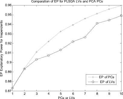
References Several cancer classifiers combined with PLS-DR for base on gene expression profile
- Alon, U. Barkai,N. Notterman,D.A. Gish,K. Ybar,S. Mack,D. and Levine,A.J. Broad patterns of gene expression revealed by clustering analysis of tumor and normal colon tissues probed by oligonucleotide arrays. Proc. Natl Acad. Sci. USA,1999;96,6745-6750.
- Boulesteix,A.-L. PLS dimension reduction for classification of microarray data. Statistical Applications in Genetics and Molecular Biology. 2004;3(1),33.
- Boulesteix A L and Strimmer K, Partial least squares: a versatile tool for the analysis of high-dimensional genomic data[J]. BRIFINGS IN BIOINFORMATICS. VOL 8.NO 1. 32~44, Jan, 2007.
- D ai,J.J. Lieu,L. and Rocke,D. Dimension reduction for classification with gene expression data. Statistical Applications in Genetics and Molecular Biology 2006;5(1), Article 6.
- Terrence S. Furey, Nello Cristianini , Nigel Duffy, David W. Bednarski , Michèl Schummer and David Haussler. Support vector machine classification and validation of cancer tissue samples using microarray expression data. Bioinformatics 2000; v16, n10, 906-914.
- J.G. Liao Khew-Voon Chin. Logistic regression for disease classification using microarray data: model selection in a large p and small n case.Bioinformatics 2007; v23, n15,1945-1951.
- Jian-Nan Zhang, A-Li luo, Yong-Heng Zhao, Automated estimation of stellar fundamental parameters from low resolution spectra: the PLS method. Research in Astonomy and Astrophysics.June 2009;V9,n6,712-724.
- Menezes,J.c. Felicio,C.C. Bras,L.P. Lopes,J.A. and Cabrita,L. Comparison of PLS algorithms in gasoline and gas oil parameter monitoring with MIR and NIR. Chemometrics and Intelligent Laboratory Systems. 28 July 2005;V78,n1-2,74-80.
- Nguyen,D.V. and Rocke,D.M., Tumor classification via partial least squares using microaray gene expession data. Bioinformatics, 2002(a),18(1),30-50.
- Nguyen,D.V. and Rocke,D.M, Multi-class cancer classification via partial least squares with gene expression profiles. Bioinformatics, 2002(b),18(9),1216-1226.
- Wold,H, Estimation of principal components and related models by iterative least squares. Krishnaiah PR (ed). Multivariate Analysis. New York: Academic Press, 1966; 391-420.
- W old,H, Nonlinear Iterative Partial Least Squares(NIPALS) modeling: some current development. Krishnaiah PR (ed). Multivariate Analysis. New York: Academic Press, 1973; 383-407.
- Wold,H, Path models with latent varibles: the NIPALS approach. Blalock HM(ed). Quantitative Sociology: Internatioanl Perpectives on Mathematical and Statistical Model Building. New York: Academic Press, 1975.
- Xue-Qiang ZengGuo-ZhengLi Geng-FengWu JackY.Yang M.Q. Irrelevant gene elimination for Partial Least Squares based Dimension Reduction by using feature probes. International Journal of Data Mining and Bioinformatics. 2009;v3,n1,85-103.
