Широтная амплитудно-фазовая структура МГД-волн: моделирование наблюдений на радаре STARE и магнитометрах сети IMAGE

Автор: Пилипенко В.А., Козырева О.В., Федоров Е.Н., Успенский М.В., Кауристи К.
Журнал: Солнечно-земная физика @solnechno-zemnaya-fizika
Статья в выпуске: 3 т.2, 2016 года.
Бесплатный доступ
Разработана численная модель, которая дает стационарное распределение компонент поля МГД-волны в неоднородном плазменном ящике, моделирующем реальную магнитосферу. Рассматривается проблема достаточного граничного условия на границе ионосфера-магнитосфера для связанной МГД-моды. Для обоснования модельных предположений в явном виде получено неравенство, показывающее, в каком случае можно пренебречь индуктивным xолловским эффектом при рассмотрении отраженной от ионосферных границ альфвеновской волны. Модель предсказывает наличие характерной особенности пространственного амплитудно-фазового распределения поля УНЧ-колебаний, которая не была замечена в работах по теории резонанса силовых линий, - существование области с противоположными фазовыми задержками на стороне источника резонанса. Этот теоретический прогноз подтверждается амплитудно-фазовой широтной структурой Рс5-пульсаций, наблюдаемых STARE радаром и IMAGE магнитометрами. Постепенное увеличение азимутального волнового числа m на меньших L -оболочках наблюдалось на долготно-разделенных радарных лучах.
Мгд-волны, геомагнитные пульсации, трансформация мод, ионосферный радар, магнитометр
Короткий адрес: https://sciup.org/142103611
IDR: 142103611 | УДК: 523.62.7266 | DOI: 10.12737/19418
Текст научной статьи Широтная амплитудно-фазовая структура МГД-волн: моделирование наблюдений на радаре STARE и магнитометрах сети IMAGE
Resonant transformation of MHD wave modes provides the physical background for diagnostics of the magnetospheric Alfven resonator (MAR) parameters using ground-based observations of ULF pulsations. Resonant features of ULF waves in the Pc3–5 bands (periods from few tens of seconds to several minutes) make it possible, though their source is unknown, to determine local values of key parameters of the MAR, such as the resonant frequency ω A which is a proxy for the magnetospheric plasma density, and the width of the ULF resonant peak δ which is an indicator of the dominant damping mechanism.
The theory of field line Alfven resonance (FLR) based on the idea of transformation of fast magnetosonic (compressional) mode into Alfven wave is one of the key theories in the physics of ULF waves in the terrestrial magnetosphere [Tamao, 1965]. According to this theoretical concept, MHD disturbances from outer magnetospheric domains propagate inside the inhomogeneous magnetosphere and through a mode transformation excite standing field line oscillations in the MAR between conjugate ionospheres. The mode conversion is the most effective in the vicinity of the resonant geomagnetic shell 56
where the frequency ω of the external source coincides with the local frequency ω A ( L ) of Alfven field line oscillations. Wave energy pumping into the resonant region causes a growth and narrowing of the spatial resonant peak. This growth terminates at a certain level depending on the dominant dissipation mechanism, such as the ionospheric Joule dissipation [Yumoto et al., 1995], leakage into a small-scale dispersive Alfven wave [Streltsov, Lotko, 1996], magnetospheric turbulence [Coult et al., 2007], or a finite time driving [Leonovich, Mazur, 1998]. The dominant damping mechanism thus determines the effective Q-factor of the MAR. The resonance width and gain can be approximated as d— a / Q and
B max /B 0 — Q , where a is the lateral scale of the Alfven velocity inhomogeneity.
The central problem of the experimental determination of the MAR parameters is that the input to the spectral content from the MAR resonant response and from the wave source is comparable. That is, the spectral peak does not necessarily correspond to ωA, and δ cannot be used directly to determine the MAR quality factor Q A . This ambiguity can be resolved with the help of the gradient method [Baransky et al., 1995] and its advanced modifications [Kawano et al., 2002]. Precise measurements of the gradients of spectral amplitude and phase along a small baseline allow one to exclude the influence of the form of the source spectrum and to reveal even relatively weak resonant effects.
Originally the basic notions of the FLR theory were formulated within the framework of an extremely simplified model: a ”plasma box” with 1D inhomogeneity across straight field lines [Southwood, 1974]. Despite the apparent simplicity of such a model, the spectral properties of the relevant system of MHD equations turned out to be non-trivial. The methods of qualitative theory of differential equations were applied to generalize the basic results for more complicated systems [Krylov et al., 1981; Kivelson, Southwood, 1986; Chen, Cowley, 1989; Fedorov et al., 1995; Klimushkin et al., 2004]: multi-dimensional inhomogeneity, curvilinear magnetic field, finite plasma pressure, and finite conductivity boundaries. The results of these studies confirmed that basic predictions of plasma box theory remain valid in a more realistic situation. For this reason, this simple box model gives an unexpectedly comprehensive description of the observed ULF resonant spatial structure from Pc5 waves at auroral latitudes [Ziesolleck, McDiarmid, 1994] to Pc4 at mid-latitudes [Green, 1978; Kurchashov et al., 1987; Fedorov et al., 1990] and Pc3 pulsations at low latitudes [Waters et al., 1991].
The main knowledge about the spatial structure of ULF waves was obtained with ground-based magnetometers. Thus, only the signals inevitably distorted by transmission through the ionosphere were available for comparison with the theoretical predictions. However, modern radar facilities provided a possibility to detect Pc5 waves in the ionosphere. STARE radar facility initiated a breakthrough in the characterization of 2D spatial structure of various types of Pc5 waves [Walker et al., 1979; Allan, Poulter, 1984]. Besides large-scale toroidal Alfven waves [Ruohoniemi et al., 1991; Yeoman et al., 1997; Ziesolleck et al., 1998; Kleimenova et al., 2010], radar observations revealed small-scale poloidal Pc5 pulsations screened by the ionosphere from ground magnetometers [Walker et al., 1982; Yeoman et al., 2000].
The FLR theory is a local theory, thus the asymptotic solutions it provides describe only the local structure in the nearest vicinity of a resonant field line. More global distribution can be described only by a numerical model, or analytically by using considerable theoretical simplifications [Fedorov et al., 1998]. A number of numerical models have been developed and successfully used to study the global MHD wave propagation in the magnetosphere. A 1D steady-state model with a realistic profile of the Alfven velocity down to very low latitudes ( L <2) was developed by Waters et al. [2000]. Time-dependent models of excitation of coupled MHD modes have been developed for cylindrical [Allan et al., 1986] and dipole [Lee, Lysak, 1989] geometries. All these models have provided many insights into the problem and have given a solid confirmation to the results obtained from the local analytical treatment. In this paper, we develop a 1D steady-state model similar to Waters et al. [2000] but will apply this model to interpret in greater detail the amplitude-phase ULF wave behavior at auroral latitudes. Predictions of this model have been validated with the data from simultaneous observations of Pc5 waves at STARE radar and ground IMAGE magnetometers. The STARE radar provides a better spatial coverage than the ground magnetometers, and this gives a possibility to reveal additional features of ULF wave latitudinal structure.
WAVE MHD MODEL OF THE MAGNETOSPHERE
In the 1D plasma box model used here, linear oscillations of a cold (в^1) plasma embedded in a magnetic box are considered, which simulates the auroral magnetosphere. Axis Z of the Cartesian coordinate system is oriented anti-parallel to the homogeneous magnetic field B0=–B0ez, axis X is directed sunward, corresponding to the dimensionless radial distance L=x/RE+1, and along the eastward direction Y the system is homogeneous. Magnetospheric plasma density N(x) is assumed to be inhomogeneous across the magnetic field providing an inhomogeneous distribution of Alfven velocity, VA(x). Dependence of the wave fields A(r, t) on the spatial coordinate and time is assumed to be « A(x)exp(-iиt+ikyy+ikzz). The combination of the MHD and Maxwell equations gives the following system of coupled wave equations [Fedorov et al., 1995]:
L A ^ y = — ik y b ,
L A ^ x =-d x b , (1)
d x ^ x + iky ^ y = b , where LA = dzz + kA denotes the Alfven operator, kA(x)=и/VA(x) is an Alfven wave number, and b=-Bz/|B0| is the normalized compressional component of wave magnetic field. The transverse plasma displacement ξ is related to the plasma velocity v as follows v=–iωξ. Components of the wave electric E and magnetic B fields can be found from the following relations:
E x / B 0 = i ωξ y , E y / B 0 = – i ωξ x , (2)
B x / B 0 =∂ z ξ x , B y / B 0 =∂ z ξ y .
The wave electromagnetic field can be imagined as a sum of two partial modes, B = B (A)+ B (F), E = E (A)+ E (F), namely:
-
(A) Alfven wave, in which the compressional component of disturbed magnetic field B^ = 0, and
-
(F) fast magnetosonic (compressional) wave, in which a disturbed field-aligned current vanishes, 58
( V B ( F ) ) e z = 0.
Mathematically, this decomposition can be done with the help of potentials for Alfven and compressional disturbances [Fedorov et al., 1998]. In a homogeneous plasma, equations (1) are decoupled and give the dispersion relationships for the Alfven mode, mA= k z V A , and compressional mode ю = ( k x + k y + k ^ ) 12 V A . A large-scale toroidal Alfven mode ( k y ^ k x ) has the dominant components B y , E x , ^ y , and no magnetic field compression B z . This mode is excited by MHD disturbances from the distant magnetosphere via the Alfven FLR. In an azimuthally small-scale poloidal Alfven mode ( k y » k x ), the dominant components are Bx , Ey , and L x . This mode is predominantly excited by magnetospheric energetic particles.
Neglecting for a moment the azimuthal variation of a wave as compared to its radial gradient, that is k y →0, one can see from (1) that the B y , ξ y components correspond to an Alfven mode, whereas the B x , ξ x and b components correspond to a compressional mode. The Alfven component should reveal resonant behavior near the singular point ω=ωA, whereas compressional components should demonstrate nonresonant behavior. Upon penetration through the ionosphere, taking into account the π/2 rotation of the wave polarization ellipse owing to the ionospheric Hall currents, the B y and B x components yield H and D components, correspondingly, of the magnetic response on the ground.
The compressional mode propagation across the plasma box magnetosphere is terminated by the reflection (turning) point, where m ^ m F = ^ k y 2 + k Z V A . Thus, the wave regime of this mode inside the magnetosphere is controlled by the radial distribution of the turning point periods T F ( x ) = T A ( x ) / ^ 1 + ( k y / kz ) . The propagation regions are those, where T < T F( x ), whereas in opaque (non-transparent) regions, where T > T F ( x ), magnetosonic waves are evanescent. The azimuthal wave structure in the magnetosphere is commonly modeled as exp( im Λ), where Λ is the longitude, and m is the azimuthal wave number. We consider large-scale modes with m ~1 which can penetrate deep into the magnetosphere.
MAGNETOSPHERIC WAVES AND THE IONOSPHERE
The magnetospheric plasma is assumed to be embedded between conjugate ionospheres at z =± L , whereas the Earth’s surface is represented as planes at z =±( L + h ), where h is the height of the ionosphere. A high but finite conductivity of the Earth has no noticeable influence on the MHD wave fields in the magnetosphere. Therefore, the Earth’s surface may be treated as an ideally conducting layer where the ULF wave horizontal components vanish, that is E τ( z =±( L + h ))=0. The transfer of this boundary condition from the Earth’s surface to the lower boundary of the ionosphere depends on the wave mode. The wave field above the ionosphere is composed from Alfven and fast modes, B ^ A ) , B ^ H ) ; and beneath it, from electric and magnetic modes B 1?1 , B ^ H ) .
In the inhomogeneous magnetosphere, MHD modes are coupled. This coupling is especially effective near the Alfven resonant shell and results in the formation of a spatially narrow amplitude peak of Alfven mode intensity. Owing to this process, spatial scales of compressional and Alfven modes are essentially different: near the ionosphere the horizontal scale of the compressional mode is ≥103 km, whereas that of Alfven mode in the vicinity of the resonant shell is ~102 km. The distinct difference between the horizontal scales of partial modes results in different boundary conditions for them.
For an electric E-mode ( B z =0, j z ≠0, E z ≠0) the atmospheric conductivity, σ a , can be important. However, as the conductance of the atmospheric column with any reasonable transverse wave scale (<104 km) is much less than the height-integrated conductance of the ionosphere, the vertical current in the atmosphere j z can be neglected. This yields the condition of current non-penetration at the lower ionospheric boundary, that is jz ( z =± L )=0. In a magnetic H-mode, the vertical electric current and field are absent, jz = Ez =0, and the atmospheric gap has no influence on this mode.
In the ULF frequency range, when the ionospheric skin-depth δ P and thickness of conductive layer ∆ h are less than the horizontal scale of disturbance, that is k τ δ P <1 and k τ ∆ h <1, the thin ionospheric sheet approximation may be used, and the ionosphere can be replaced by a thin sheet with a tensor of height-integrated anisotropic conductance T [Alperovich, Fedorov, 2007].
In general, upon the incidence of the Alfven mode onto the anisotropic ionosphere, the Alfven and fast modes are coupled due to the Hall conductance. However, for a sufficiently small transverse scale, the Alfvenic part of wave disturbance decouples from a fast mode, so the latter mode does not influence the Alfven wave reflection. In the Appendix, we derive a strict condition under which the influence of the Hall inductive effects can be neglected. This condition may be violated for a high wave frequency ω or large ionospheric Hall conductance. In such a case, the ground signal will be additionally reduced compared with that above the ionospheric conductive layer. This reduction may be interpreted as the inductive shielding effect [Yoshikawa, Itonaga, 1996] or as an energy loss due to excitation of the surface-type gyrotropic wave in the ionosphere [Pilipenko et al., 2000]. The inductive Hall effect may be significant for the Pc3 transmission through the dayside ionosphere at low latitudes [Sciffer, Waters, 2002; Sciffer et al., 2004] and can influence the eigenfrequency of the MAR [Waters, Sciffer, 2008].
When the inductive Hall effect is neglected, the ionospheric boundary condition for the Alfvenic wave disturbance is as follows
7 < A)=-vT ( £ e . । , (3)
where VT=V- z V is the horizontal projection of the operator V . Assuming that the ionospheric conductance is laterally homogeneous, relationship (3) can be re-written using Faraday’s law as an impedance-type relationship B ( T A ) = p 0 T P E ( T A ) n , where n is a unit vector normal to the ionosphere. According to this relationship, the height-integrated Pedersen conductance Σ P plays the role of the ionospheric surface admittance for Alfven waves. The damping rate γ and quality-factor Q A of Alfven 60
wave n -th harmonic is determined by the ratio between Σ P and the wave admittance of the magnetosphere Σ A =1/µ 0 V A [Yumoto et al., 1995], namely
— = ±ln I p -I a , Q = . (4)
to n n I P + I A A 2 y
For a partial H-mode (comprising fast mode in the magnetosphere and magnetic mode in the atmosphere) the jumps of horizontal electric and magnetic components across the conductive ionospheric layer { ( B , E )^ } = ( B , E ) ( T F ) - ( B , E ) T H ) are
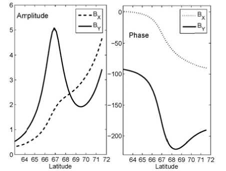
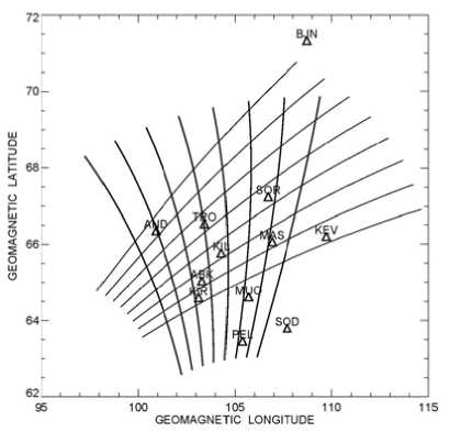
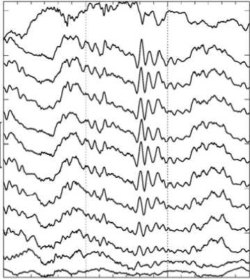
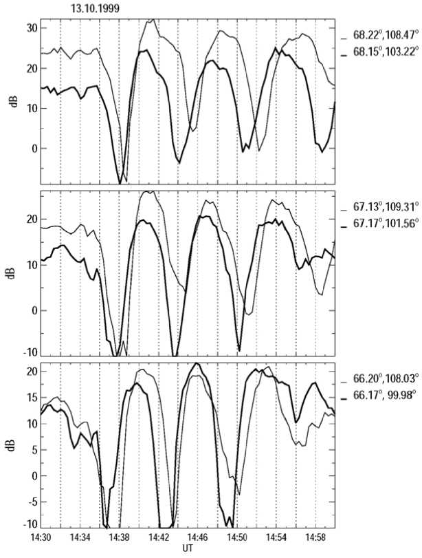
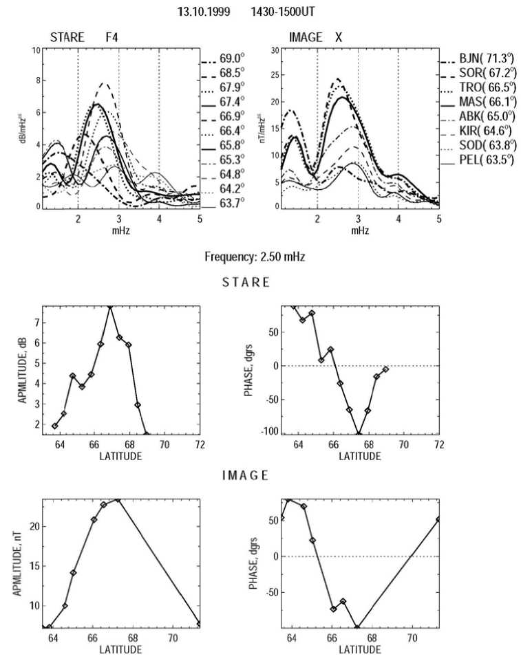
{E From (5) the ionospheric boundary condition for a fast mode stems B(F) = —— Г(1 + itoц0IP h)E(F)n + itoц0IhhE(F)1.(6) i to h LJ In the Pc5 band, both for dayside and nightside conditions, wu0hEP,H ^ 1. Hence, from (6) the simplified boundary condition follows [Hameiri, Kivelson, 1991] B(TF)= — E(TF)n.(7) i to h Thus, the reflection of a fast compressional mode is mainly determined not by the ionospheric conductance, but by the altitude h of the ionosphere above the ground, and the reflection of this mode from the ground in the ULF frequency range is very high. Indeed, the comparison between the fast mode impedance ZF= toц0 / ^kA + k2~ -iц0to/ k and the ionospheric surface impedance Zi~iюц0h/(1+ i®ЦоhSP) gives |Z|/ZF|< kh^1. Thus, the wave impedance of the fast mode is much less than the ionospheric surface impedance, and for this mode the system ionosphere–ground can be modeled as an ideal conductor. It is not evident what kind of boundary condition is to be used for coupled MHD modes [Hameiri, Kivelson, 1991]. Under dayside conditions EA^EP, the ionosphere is nearly a perfect reflector for an Alfven mode. For a compressional mode the system ionosphere–atmosphere–ground is a perfect reflector too. In the vicinity of the resonant shell, where the wave energy enhancement/absorption occurs, the magnetospheric wave field is dominated by the Alfven mode contribution. As a result, for the dayside ionosphere the boundary condition for total fields B=B(A)+B(F) and E±=E(A)+E(F) may be adapted in the same form as for the Alfven wave BΤ= µ0ΣPEΤN. (8) Here we cite the necessary relationships which couple the magnetic disturbance above the ionosphere, ionospheric electric field disturbance (measured by radars), and ground magnetic response (recorded by magnetometers). Upon the transmission of Alfvenic toroidal mode (ky→0) through the ionosphere, the wave ellipse rotation should occur By ^ B^ (H-component), Bx ^ By8’ (D-component). Neglecting the ionospheric inductive effect and finite ground conductivity, the wave spatial spectrum near the ground B.'8) (k) is related to the spatial harmonic of magnetic disturbance in the ionosphere BУg)by the relationship B^ (kx ) = By (kx ) |H sin I exp (-kxh ) , XP where I is the magnetic field inclination. In the vicinity of the Alfven resonant shell (x—x0), the ground spatial structure of magnetic disturbance Bx®’ (x) is found by the inverse Fourier transform of magnetospheric resonant structure By(x)=iB(m)δ/(x–x0–iδ) [Pilipenko et al., 2000] i 5 x - x0 - i (5 + h)’ B(g) (x) — B(m) ^Hsin I X where B(m) is the peak value of resonant structure. Thus, the ground magnetic response to the resonant structure has the same spatial form as an incident wave, but the peak amplitude at x→x0 is reduced by the factor (ΣH/ΣP)sinIδ/(δ+h), and the peak width is smeared (δ+h)/δ times. If the Alfvenic structure is not very narrow, δ>h, the relationship between the ionospheric disturbance and ground response is B^ — Bym) (XH / XP) sin I. The ionospheric electric field induced by a large-scale (kxh<1, ky→0) Alfven mode is related to its ground magnetic response as [Pilipenko et al., 2012] Ex =-(Цо XHsin 1 )-1 Bxs), (9) where µ0=4π∙10–7 H/m is the magnetic constant. To stimulate the plasma turbulence and cause backward reflection of the STARE radar sounding signal, an electric drift velocity must be higher than the threshold value V—20 m/s which corresponds to ionospheric electric field E —1 mV/m [Walker et al., 1979]. According to estimate (9) in the daytime (SH=10 S) high-latitude (I—90°) ionosphere, an Alfven wave with the magnetic response on the ground B^ > 12 nT is sufficient to induce the backscatter process in the ionosphere. Though modeling boundary condition (8) does not provide an exact dissipation rate of the compressional mode, this condition, as well as more exact condition (7), indicates a very low damping of this mode. Here we are mainly interested in the wave structure near the daytime resonant shell, where the Alfven component with boundary condition (8) dominates. Thus, though a MHD wave in a realistic inhomogeneous magnetosphere is a coupled Alfven and fast mode, the same boundary condition in the ionosphere can be used for this mode as for the pure Alfven mode during numerical modeling. NUMERICAL MODEL The 1D model discussed here is restricted to high latitudes (vertical B0). Our numerical code calculates the steady-state distribution along L of the wave transverse displacements ξx, ξy, the magnetic components Bx, By, and the normalized field-aligned component of wave magnetic field b, excited by a harmonic source with the frequency ω at the magnetopause. The model calculates the field-aligned wave structure in the plasma box with finite-conductive boundaries, and provides magnitudes of magnetic components just above the ionosphere. The azimuthal wave vector ky is chosen by fitting the azimuthal wave number m at certain L, ky=m/LRE. At the magnetopause (LMP), the boundary condition is imposed as follows Sx (L = LMP ) = ^ (z) exp (-i®t + ikyy ) (10) corresponding to a magnetopause radial displacement with the amplitude ξ(0). In the near equatorial ionosphere, the boundary condition ξx(L=1)=0 is imposed. A radial distribution of the Alfven period TA(L) is modeled in the following way. Several key values of TA(L) are chosen to fit a desired profile, then a smooth continuous function is reconstructed with the spline interpolation. The chosen profile TA(L) comprises the plasmapause at L=4, but its occurrence does not influence the wave structure in the considered range of auroral latitudes. The magnetospheric wave conductance ΣA for each field line is determined by local Alfven velocity; and the ratio between ΣA and ΣP determines MAR dissipative properties (4). The Alfven period is determined by the length of field line Lz and plasma density N. For correspondence with the realistic dipole geometry the nominal field line length can be calculated at each L as follows Lz (L) = LRE Ц1 -L-1)(4-3L-1) + -13log(3(1 -L-1) + \4-3L-1)(11) For L>2 instead of (11) a simpler relationship can be used Lz—2.76L-2.0. The ’’apparent” Alfven velocity is calculated from a given TA and Lz as VA=2Lz/TA. The resulting profile of TA is a good approximation to reality, but the derived value of VA may differ noticeably from the realistic ones due to the over-simplicity of the magnetic field geometry. The radial distribution is converted into the latitudinal distribution with the relation L=cos–2Φ. MHD WAVE STRUCTURE IN THE MAGNETOSPHERE: MODELING RESULTS The model radial distribution of the parameters of MAR, namely, Alfven period, and apparent Alfven velocity throughout the magnetosphere are shown in Figure 1. The ratio EP/EA^25 is chosen to reproduce a plausible resonance curve. In the presented calculations, it is assumed that m=3 at L=6.6. The fundamental field-aligned harmonic (n=1) is considered. The resonant period TA(Φ) has been set to vary in the range Φ=64°–72° from ~350 to ~460 s. For the selected set of parameters the frequencies are below the cut-off frequencies for a compressional mode, T>TF. Therefore, the evanescent regime for a compressional mode is to be observed throughout the entire magnetosphere, and no cavity wave can be formed. Thus, the wave energy is tunneled from the magnetopause towards the resonant magnetic shell. Owing to the large scale of disturbance, even the evanescent mode transports significant wave energy into the inner magnetosphere. We consider the wave structure excited by a harmonic source with a period T=400 s (f=2.5 mHz) and unit amplitude ^x0) = 1RE. The FLR occurs at the resonant magnetic shell at Ф=67°. Figure 2 shows the radial structure of the amplitude (left-hand panel) and phases (right-hand panel) of the transverse components Bx and By in the magnetosphere. The resonance at Ф~67° reveals itself as the amplitude local peak and steep phase variations of By component. The phase variation across the resonant region Аф~120° can be seen clearly. The apparent phase velocity in the region of phase gradient is directed poleward, towards higher L. At the same time, the compressional component Bz demonstrates only a weak amplitude enhancement and phase variations in the resonant region (not shown). The amplitude of nonresonant Bx component shows no enhancement in the resonant region, but a drop behind the resonant point. The behavior of all the components in the vicinity of the resonant shell is well interpreted by the analytical FLR theory. Figure 1. Plasma-box model of the magnetosphere in the range of geomagnetic latitudes Φ=63°–72°: Alfven period TA (solid line, the scale on the left-hand axis), and Alfven velocity VA (dashed line, the scale on the right-hand panel) Figure 2. MHD wave (T=400 s) structure in the magnetosphere in the range of geomagnetic latitudes Φ=63°–72°: amplitudes in arbitrary units (left-hand panel) and phases in degrees (right-hand panel) of the Bx and By components 64 However, there is a new feature beyond the classical FLR theory: the existence of a region with anomalous phase gradient (apparent propagation velocity towards low L-shells). The anomalous phase gradient of the resonant component By is formed on the northward side of the resonant structure at ф~70°. While the phase change across the resonant region is ~120°, the anomalous phase variation northward from the Alfven resonance is ~50°. Such non-monotonic 11 variations of phase poleward of each resonant shell can be seen also in the results of Waters et al. [2000], but the authors did not discuss this effect. STARE AND MAGNETOMETER OBSERVATIONS To verify the predictions of the theoretical model, we analyze the Pc5 pulsation event detected simultaneously by the network of ground magnetometers and STARE radars on October 13, 1999. Figure 3 shows in geomagnetic coordinates the ionospheric mapping of eight beams of the Finland/Norway STARE radars as well as the position of selected stations from IMAGE magnetometer array. A short-lived, but clear, Pc5 wave packet was observed along the IMAGE meridional profile at 14:30–15:00 UT (Figure 4). The signal is most evident in the x-component, whereas in the y-component it is hardly discernible (not shown). Such asymmetry between two horizontal magnetic components is typical for a toroidal mode. The waveforms of Pc5 pulsation as detected by STARE beams at various latitudes and longitudes are shown in Figure 5. To compare the ground-based observations of Pc5 pulsations with the radar measurements, we use the 4-th beam of the Finnish radar oriented along the 105° geomagnetic meridian. At small and large distances from the radar, signals are strongly distorted due to aspect effects (a radar beam is not orthogonal to a magnetic field line at the altitude of the ionospheric E region). The measurements at Φ=64°– 69° are most reliable. Figure 6 shows the amplitude spectra of geomagnetic pulsations along the latitudinal profile of IMAGE stations (upper right-hand panel) and spectra of ionospheric variations along the STARE radar view (upper lefthand panel). Figure 3. Trajectories of the Finnish F1-F8 (thick solid line) and Norwegian N1-N8 (thin solid line) STARE radar beams in geomagnetic coordinates. Locations of IMAGE magnetometer stations are shown by triangles. The F4 beam has been used for the analysis of the ULF latitudinal structure BJN (71.3°, 108.7) SOR (67.2°, 106.7) TRO (66.5°, 103.4) AND (66.4°, 100.9) KEV (66.2°, 109.7) MAS (66.1°, 106.9) KIL( 65.8°, 104.3) ABK (65.0°, 103.3) KIR (64.6°, 103.1) SOD (63.8°, 107.7) OUJ (60.9°. 106.5) NUR (56.6) 103.0) 13 14 15 16 ut Figure 4. Pc5 wave packet detected by the IMAGE array (x-component) on October 13, 1999 at 13–16 UT. The geomagnetic latitudes and longitudes of each station are indicated near the right-hand Y-axis Figure 5. Waveforms of ionospheric disturbance (in dB) from longitudinally separated pairs of STARE beams (indicated in the panel title) at different geomagnetic latitudes (indicated near the right-hand axis) Figure 6. Amplitude spectra of ionospheric variations as measured by STARE (upper left-hand panel) and geomagnetic pulsations (upper right-hand panel) as measured along the IMAGE array on October 13, 1999 (14:30– 15:00 UT). The codes and geomagnetic latitudes of the radar range bins (from 495 to 1200 km from the radar at an interval of 15 km) and stations are shown near the right-hand axis. Middle panels show the latitudinal distribution of the ionospheric amplitude and phases at the frequencies of the spectral maximum T=400 s. The same for the ground magnetic pulsations is shown in the bottom panels A maximum centered at 2.5 mHz is registered in the pulsation spectra both by ground magnetometers and the radar. At this frequency, the latitudinal distributions of the wave amplitude and phase in the ionosphere (middle panels) and on the ground (bottom panels) have been calculated. Both ionospheric pulsations and ground magnetic variations have the local maximum in latitudinal distribution around 67°. Approximately in the same region, 65°–67°, their phases show a steep gradient ~170° for ionospheric pulsations and ~150° for ground magnetic pulsations. Besides this gradient, which is a typical signature of FLR, one can see the existence of a region with anomalous phase variations on the northward 67 side of the amplitude peak. The phase variations in this region are ~100° in the radar data. Owing to the large magnetometer gap between 67° and 72°, the northern part of the Pc5 spatial structure cannot be described with sufficient accuracy. Nonetheless, the amplitude/phase data from the BJN station indicate the occurrence of a phase gradient opposite to the resonant gradient. The azimuthal wave number has been estimated by the comparison of records of radar beams at the same latitude, but with separation ∆Λ in longitude (Figure 5). The cross-correlation time shift ∆τ between the pair of beams has been used to determine the azimuthal wave number: m=360°∆τ/T∆Λ for a wave with a period T=400 s. The calculation results for different latitudes are as follows: Φ=66.2°: ∆Λ=8.0°, ∆τ=40 s, and m=4.5, Φ=67.1°: ∆Λ=7.8°, ∆τ=40 s, and m=4.6, Φ=68.2°: ∆Λ=5.3°, ∆τ=60 s, and m=10.2. Thus, the dominant m-value decreases from ~10 at 68° to ~5 at 66°. The cause of this effect is probably diminishing of a relative contribution of higher m-values into the structure of ULF waves upon the transmission into the deeper regions of the magnetosphere. However, it should be taken into account that upon the determination of m-value from longitudinally separated observations the meridional phase gradient may influence the results because even a small misalignment between the FLR contour and station’s location may cause noticeable deviations of phase differences. Though the results of the azimuthal wave number determination should be considered with caution, we should like to indicate that the dependence of m-value on latitude, m(Φ), has not been previously reported. ESTIMATES OF THE PC5 E-FIELD MAGNITUDES COMBINING THE EISCATAND STARE OBSERVATIONS During the event under consideration, the EISCAT radar was run with Tromsø antenna being pointed along the local magnetic field line and the Kiruna and Sodankylä receiver beams being oriented toward a common volume at a height of ~280 km. Such a configuration of the EISCAT beams allows us to perform tri-static electric field measurements. From EISCAT data the mean values of the ionospheric height-integrated conductances during the interval under study were estimated to be EH—4 S and EP—3.5 S. The conductances exhibit weak periodic oscillations, with peak-to-peak amplitudes AEH—2 S and EP—1 S, caused by modulation of the ionospheric density by Pc5 wave. Pc5 pulsations seen in the EISCAT and STARE data exhibit a reasonable similarity (not shown). Periodic echo amplitudes are seen at different slant ranges (latitudes): stronger pulsations in Norway STARE radar cover an area 100–300 km northward from the EISCAT. Weaker pulsations are visible in a wider interval of distances from ~550 to ~1000 km. In Finland, STARE radar similarly structured pulsations with about three times weaker amplitudes occur, which cover the distances from ~550 to ~1200 km. Both the range profiles exhibit a gradual phase shift of the Pc5 pulsation amplitudes as a 68 function of latitude. The effective electron densities also show pulsations, which are a result of the ionospheric modulation by Pc5 wave. Although there is a factor which we have to keep in mind: a 2.5-order difference between the EISCAT and STARE collected areas. The E-field pulsations in the interval 14.6–14.9 UT have magnitudes up to ~40 mV/m in respect to their mean value of 47.5 mV/m. The STARE backscatter amplitudes react nearly linearly to the E-field pulsations [Uspensky et al., 2011], and we can use this feature for calibration. The basic parameter which defines properties of scattering media is the backscatter volume cross section (VCS). It is a relative difference between the incident power falling at a unit volume and a power which the volume as a secondary isotropic scatterer able to radiate outside through the surface of the unit sphere. The widely accepted equation for VCS (e.g., Uspensky et al. [2011] and references therein) is Ge = 32n2re2N2((5N/N)2) f (k), (12) where re is the classical electron radius, N is the backscatter volume mean electron density, and f(k) is the 3D normalized spatial fluctuation power spectrum. If one knows the electron density N in the backscatter volume, then the rms fluctuation amplitude can be found from (12). For the case under consideration we can solve (12) in absolute values since we have the effective electron density in the EISCAT flux tube. However, outside of the EISCAT volume all STARE pulsation samples have no independent information on a local volume ionization. The backscatter amplitudes, which we are using to estimate the electric field pulsations, can be expressed quantitatively from (12). The backscatter amplitude depends linearly on the rms electron density fluctuation amplitude ((6N/N)2))1/2 and the mean electron density N in the backscatter volume. The electric fields measured by the EISCAT with 1 min temporal resolution most probably somewhat underestimated the pulsation magnitudes. A reasonable estimate of the pulsation peak magnitude regarding its mean, we believe, has to be between 25 and 30 mV/m. The influence of the electron density in the backscatter volume is accounted by normalizing the backscatter pulsation amplitude by the mean backscatter amplitude preceded the first peak of the pulsations. We suggest also that the mean electron density fluctuation amplitude, ((dN/N)2)12, reacts at the electric field magnitudes >25 mV/m nearly linearly [Uspensky et al., 2011]. If the positive peaks of Pc5 pulsations at EISCAT are 25–30 mV/m, then the pulsation at Φ=68.5° can be estimated as 35–42 mV/m. The calibrated peak-to-peak E-field of Pc5 waves is about 40 mV/m. At the same time, the ground magnetic peak-to-peak amplitude is ~140 nT. Therefore, the apparent admittance is X = Bf' / ц0Ex ~ 0.8 -140/ 40 ~ 3 S. The theory of MHD wave interaction with the thin-layer ionosphere predicts that for a large-scale (m→0) Alfven wave the impedance is to be X(A)=ZH/sin/~4 S. Thus, the observed apparent admittance is very close to the theoretically predicted one for the incident toroidal Alfven wave determined by the ionospheric height-integrated Hall conductance from EISCAT data. DISCUSSION To illustrate the effect of the anomalous phase gradient formation, one must go beyond the leading term of the asymptotic decomposition of the coupled MHD equations in the vicinity of a resonant field line. For a linear radial profile of plasma parameters, an analytical solution for the coupled wave structure in the plasma box model can be obtained [Southwood, 1974]. For the resonant magnetic component By this solution, decaying deep into the magnetosphere (x→–∞), reads By (x, f) ∝ K1(–ky(x–x0–iδ)), (13) where K1 is the modified Bessel function of the second kind. On the source side of the Alfven resonance point, solution (13) has the following form By(x>x0, f)∝–K1(ky(x–x0–iδ))–iπI1(ky(x–x0–iδ)), (14) where I1 is the modified Bessel function of the first kind. Though in this region the compressional modes are evanescent, the first term in (14) may be imagined as a wave incident on the resonant point, whereas the second term corresponds to the wave reflected from the resonance point (its amplitude decays exponentially away from the resonance x>x0). Considering the asymptotic behavior of Bessel functions at large |kyx|, one can see that the wave incident on the resonance point reflects from it with the phase shift π/2. The interference of ”incident” and ”reflected” components produces the anomalous phase behavior. The effects under discussion should provide distortions of the amplitude and phase gradients measured along the latitudinally separated stations (gradient method). These features will be revealed in asymmetric forms of gradient plots, ∂xA(f) and ∂xφ(f). These predictions are to be verified by detailed analysis of gradient measurement data. Also, the model predicts that a substantial drop of non-resonant D component may occur just equatorward of the resonant shell. However, even a small leakage of more powerful H component into weak D component may obscure this effect during ground observations. A more reliable interpretation of this feature requires a more advanced numerical model of the MAR, comprising a dipole or more advanced geomagnetic field, e.g., the 2D model of Waters and Sciffer, [2008] or the 3D model of Lee, Lysak [1989]. In the 1D model considered, the field-aligned structure of both MHD modes is a simple standing sinusoidal wave. In a realistic magnetosphere, the bulk of the fast magnetosonic oscillation energy tends to concentrate in a low-VA region near the magnetospheric equatorial plane [Leonovich, Mazur, 2000]. Therefore, the efficiency of the mode coupling is to be different for different field-aligned wave structures. Here only two MHD modes pertinent to a cold plasma have been considered. When small, but finite, plasma pressure is taken into account, the resonant conversion of fast magnetosonic waves into slow magnetosonic oscillations becomes feasible [Leonovich et al., 2006], though magnetospheric slow magnetosonic oscillations cannot be observed on the ground. In a magnetosphere with a dipole-like magnetic field, monochromatic fast waves were shown to drive, standing along magnetic field lines, slow magnetosonic oscillations, narrowly localized across and along the geomagnetic field lines. In a finite-pressure plasma (e.g., in the outer magnetosphere), the poloidal Alfvenic mode is coupled with the slow magnetosonic mode into ballooning mode [e.g., Agapitov et al., 2007]. CONCLUSION Besides classical resonant effects, such as the amplitude peak and extreme phase gradient of H component at the resonant latitude, the plasma-box model predicts a new feature of the ULF wave meridional structure: the occurrence of the ”opposite” phase gradient on the northward (outward) side of FLR. This prediction has been confirmed by the synchronous STARE radar and magnetometer observations of Pc5 pulsations. This research is supported by the RFBR grant 14-05-00588 (VP, EF), and the grant 246725 from the POLARPROG program of the Norwegian Research Council (OK). APPENDIX: NECESSITY TO ACCOUNT FOR THE IONOSPHERIC HALLINDUCTIVE EFFECT Here we provide a strict criterion for determining cases when the influence of the Hall inductive effect could be neglected. The Alfven wave damping in the ionosphere, and consequently the width of the resonant response, are determined by the factor 1–RAA, where RAA is the Alfven wave reflection coefficient. For the vertical geomagnetic field B0 the comparison of the classical RAA and the additional term caused by the Hall inductive effect [Yoshikawa, Itonaga, 1996; Yagova et al., 1999; Alperovich, Fedorov, 2007] gives the condition when the latter effect is insignificant < 2 Za(+ za ) GW Zp I Zp J kah , where the function G(z)=z(1–exp(–z))–1. For a wide resonance (kh<1) at dayside (ΣP>ΣA) condition (15) is reduced to Z. Y ^ 2 Za 1 (Zp J Zp kA h In the Pc5 range (T=300 s), condition (16) is fulfilled for the dayside ionosphere (EA/EP~0.1, FA~500 km/s) when (EH/SP)2^40. Thus, for dayside Pc5 waves the Hall inductive effect can be neglected in the ionospheric boundary conditions.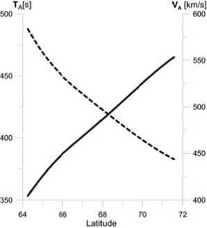

Список литературы Широтная амплитудно-фазовая структура МГД-волн: моделирование наблюдений на радаре STARE и магнитометрах сети IMAGE
- Agapitov A.V., Cheremnykh O.K., Parnowski A.S. Ballooning perturbations in the inner magnetosphere of the Earth: spectrum, stability and eigenmode analysis. Adv. Space Res. 2007, vol. 41, pp. 1682-1687.
- Allan W., Poulter E.M. The spatial structure of different ULF pulsation types: A review of STARE radar results. Rev. Geophys. 1984, vol. 22, pp. 85-97.
- Allan W. White S.P., Poulter E.M. Impulse excited hydromagnetic cavity and field line resonances in the magnetosphere. Planet. Space Sci. 1986, vol. 34, pp. 371.
- Alperovich L.S., Fedorov E.N. Hydromagnetic waves in the magnetosphere and the ionosphere. Ser. Astrophysics and Space Science Library. 2009, vol. 353, XXIV, 418 p.
- Baransky L.N., Green A.W., Fedorov E.N., et al. Gradient and polarization methods of ground-based monitoring of magnetospheric plasma. J. Geomag. Geoelectr. 1995, vol. 47, pp. 1293-1309.
- Chen L., Cowley S.C. On field line resonance of hydromagnetic Alfven waves in dipole magnetic field. Geophys. Res. Lett. 1989, vol. 16, pp. 895-897.
- Coult N., Pilipenko V., Engebretson M. Suppression of resonant field line oscillations by a turbulent background. Planetary Space Sci. 2007, vol. 55, pp. 694-700.
- Fedorov E.N., Belenkaya B.N., Gokhberg M.B., et al. Magnetospheric plasma density diagnosis from gradient measurements of geomagnetic pulsations. Planet. Space Sci. 1990, vol. 38, pp. 269-272.
- Fedorov E.N., Mazur N.G., Pilipenko V.A., Yumoto K. On the theory of field line resonances in plasma configurations. Physics of Plasmas. 1995, vol. 2, pp. 527-532.
- Fedorov E., Mazur N., Pilipenko V., Yumoto K. MHD wave conversion in plasma waveguides. J. Geophys. Res. 1998, vol. 103, pp. 26595-26605.
- Green C. Meridional characteristics of Pc4 micropulsations event in the plasmasphere. Planet. Space Sci. 1978, vol. 26, pp. 955.
- Hameiri E., Kivelson M.G. Magnetospheric waves and the atmosphere-ionosphere layer. J. Geophys. Res. 1991, vol. 96, pp. 21125-21134.
- Kawano H., Yumoto K., Pilipenko V.A., et al. Restoration of continuous field line eigenfrequency distribution from ground-based ULF observations. J. Geophys. Res. 2002, vol. 107, SMP 25 1-12.
- Kivelson M.G., Southwood D.J. Coupling of global magnetospheric MHD eigenmodes to field line resonances. J. Geo-phys. Res. 1986, vol. 91, pp. 4345-4351.
- Kleimenova N.G., Kozyreva O.V., Vlasov A.A., et al. Afternoon Pc5 geomagnetic pulsations on the Earth's surface and in the ionosphere (STARE radars). Geomagnetism and Aeronomy. 2010, vol. 50, pp. 329-338.
- Klimushkin D.Yu., Mager P.N., Glassmeier K.-H. Toroidal and poloidal Alfven waves with arbitrary azimuthal wave numbers in a field pressure plasma in the Earth's magnetosphere. Ann. Geophys. 2004, vol. 22, pp. 267-288.
- Krylov A.L., Lifshitz A.E., Fedorov E.N. About resonant properties of the magnetosphere. Izv. AN SSSR, Fizika Zemli, . 1981, vol. N6, pp. 49-59.
- Kurchashov Yu.P., Nikomarov Ya.S., Pilipenko V.A., Best A. Field-line resonance effects in a local meridional structure of mid-latitude geomagnetic pulsations. Annales Geophysicae. 1987, vol. 5A, pp. 147-154.
- Lee D.-H., Lysak R.L. Magnetospheric ULF wave coupling in the dipole model: the impulsive excitation. J. Geophys. Res. 1989, vol. 94, pp. 17097-17104.
- Leonovich A.S., Mazur V.A. Standing Alfven waves with m>>1 in axisymmetric magnetosphere excited by a non-stationary source. Annales Geophysicae. 1998, vol. 16, pp. 914-920.
- Leonovich A.S., Mazur V.A. Structure of magnetosonic eigenoscillations of an axisymmetric magnetosphere. J. Geophys. Res. 2000, vol. 105, pp. 27707-27716.
- Leonovich A.S., Kozlov D.A., Pilipenko V.A. Magnetosonic resonance in a dipole-like magnetosphere. Annales Geophysicae. 2006, vol. 24, pp. 2277-2289.
- Pilipenko V., Vellante M., Fedorov E. Distortion of the ULF wave spatial structure upon transmission through the ionosphere. J. Geophys. Res. 2000, vol. 105, pp. 21225-21236.
- Pilipenko V., Belakhovsky V., Kozlovsky A., et al. Determination of the wave mode contribution into the ULF pulsations from combined radar and magnetometer data: Method of apparent impedance. J. Atm. Solar-Terr. Phys. 2012, vol. 77, pp. 85-95.
- Ruohoniemi J.M., Greenwald R.A., Baker K.B., Samson J.C. HF radar observations of Pc 5 field line resonances in the midnight/early morning MLT sector. J. Geophys. Res. 1991, vol. 96, pp. 1569715710, DOI: 10.1029/91JA00795
- Sciffer M.D., Waters C.L. Propagation of ULF waves through the ionosphere: Analytic solutions for oblique magnetic field. J. Geophys. Res. 2002, vol. 107, 1297. DOI: 10.1029/2001JA000184.
- Sciff M.D., Waters, C.L., Menk, F.W. Propagation of ULF waves through the ionosphere: Inductive effect for oblique magnetic field. Annales Geophysicae. 2004, vol. 22, pp. 1155-1169.
- Southwood D.J. Some features of field line resonances in the magnetosphere. Planet. Space Sci. 1974, vol. 22, pp. 483-491.
- Streltsov A., Lotko W. The fine structure of dispersive, nonradiative field line resonance layers. J. Geophys. Res. 1996, vol. 101, pp. 5343-5358.
- Tamao T. Transmission and coupling resonance of hydromagnetic disturbances in the non-uniform Earth's magnetosphere. Science Rep. of the Tohoku Univ. Ser. 5. Geophysics. 1965, pp. 43-72.
- Uspensky M.V., Janhunen P., Koustov A.V., Kauristie K. Volume cross section of auroral radar backscatter and RMS plasma fluctations inferred from coherent and incoherent scatter data: a response on backscatter volume parameters, Ann. Geophys., 2011, vol. 29, pp. 1081-1092.
- Walker A.D.M., Greenwald R.A., Stuart W.F., Green, C.A. STARE auroral radar observations of Pc5 geomagnetic pulsations. J. Geophys. Res. 1979, vol. 84, pp. 3373-3388.
- Walker A.D.M., Greenwald R.A., Korth A., Kremser G. STARE and GOES 2 observations of a storm time Pc5 ULF pulsation. J. Geophys. Res. 1982, vol. 87, pp. 9135-9146.
- Waters C.L., Menk F.W., Fraser B.J. The resonant structure of low latitude Pc3 geomagnetic pulsations. Geophys. Res. Lett. 1991, vol. 18, pp. 2293.
- Waters C.L., Harrold B.G., Menk F.W., et al. Field line resonances and waveguide modes at low latitudes 2. A model. J. Geophys. Res. 2000, vol. 105, pp. 7763-7774.
- Waters C.L., Sciffer M.D. Field line resonant frequencies and ionospheric conductance: Results from a 2-D MHD model. J. Geophys. Res. 2008, vol. 113, p. A05219. DOI: 10.1029/2007JA012822.
- Yagova N., Pilipenko V., Fedorov E., et al. Influence of ionospheric conductivity on mid-latitude Pc3-4 pulsations. Earth, Planets and Space. 1999, vol. 51, pp. 129-138.
- Yeoman T.K., Wright D.M., Robinson T.R., et al. High spatial and temporal resolution observations of an impulse-driven field line resonance in radar backscatter artificially generated with the Tromsø heater. Ann. Geophysicae. 1997, vol. 15, pp. 634-644.
- Yeoman T.K., Wright D.M., Chapman P.J., Stockton-Chalk A.B. High-latitude observations of ULF waves with large azimuthal wavenumbers. J. Geophys. Res. 2000, vol. 105, pp. 5453-5462.
- Yoshikawa A., Itonaga M. Reflection of shear Alfven waves at the ionosphere and the divergent Hall current. Geophys. Res. Lett. 1996, vol. 23, pp. 101-104.
- Yumoto K., Pilipenko V., Fedorov E., et al. The mechanisms of damping of geomagnetic pulsations. J. Geomag. Geoelectr. 1995, vol. 47, pp. 163-176.
- Ziesolleck C.W.S., McDiarmid D.R. Auroral latitude Pc5 field line resonances: quantized frequencies, spatial characteristics, and diurnal variation. J. Geophys. Res. 1994, vol. 99, pp. 5817-5830.
- Ziesolleck C.W.S., Fenrich F.R., Samson J.C., McDiarmid D.R. Pc5 field line resonance frequencies and structure observed by SuperDARN and CANOPUS. J. Geophys. Res. 1998, vol. 103, pp. 11771-11785.
