Short Term Electrical Load Forecasting Based on Weather Parameters under Multiple FIS of Processing

Electrical power is now considered as the source of production of modern industrial society of the world. In Bangladesh power generating stations are interconnected to the backbone power links called national grid. Daily total power generation depends on demand of subscribers of the country. Since electrical power cannot be stored or reserved for future use, therefore difference between generation and demand should be as low as possible. Load forecasting is a method used by energy or power service providers to forecast the amount of energy or power required to maintain the equilibrium between supply and demand. Load forecasting is required to take decisions about system growth from the data of daily load demand. The forecasting of electrical load is divided into two categories: long-term and short-term. The former deals with demand-supply adjustments for periods of 10 to 50 years, while the latter does so for periods of a few months to five years. In this research work, daily electrical load of Bangladesh is used to forecast short-term electrical load. Recent literature encompasses several noteworthy contributions in electricity load forecasting. This section lists some earlier works that are pertinent to anticipate short-term electrical load. In [1], electricity loss is calculated from short-term load forecasting, where authors used fuzzy logic on historical data creating own fuzzy rules. For the forecast of the output load, five triangular MFs are used for the input variables. To process the input data and to provide an output, the fuzzy inference system is used under ‘if then’ condition. Finally, comparison is made graphically between the actual load in MW and the forecasted load, where the inaccuracy ranges from +12.14% to -9.48%.

Table 1. Few papers pertinent to this research work

Papers	Algorithm	Results	Limitation
[11]	Short-term electrical load forecasting is done training an artificial neural network (ANN) by two years data from 2016 to 2018 of energy cooperative (AEC) of Malaysia.	The paper measures the testing mean absolute percentage error (MAPE) changing the number of hidden layers (two and three) and also changing the activation functions (Tanh, Sigmoid, Softsign and Exponential). The ‘Tanh’ and ‘two hidden layers model’ reveal the best result results on both training and test data.	Only ANN is used for entire analysis.
[12]	Four regional annual load demand of Taiwan from 1981 to 2000 is applied on three algorithms: SVRIA, SVMG and ANN for training.	The MAPE in % is evaluated on testing data, where ANN gives the best results on the data of northern regional, SVRIA for other three regions: southern, eastern and central regional data.	Limited number of MLs are found for comparison.
[13]	The paper deals with complexities of different generation modalities (DGM) in long, medium, and shortterm load forecasting.	It is a review paper provides strength and weakness of machine learning algorithms: regression, SVM, ANN, RNN, LSTM, FA-SVM, ARIMA etc. A summary of previous works relating MAPE %, type of power station (Hydro, Gas, Nuclear, Diesel), applications (residential, commercial, industrial), weather parameters (temperature, wind speed, humidity) is shown in results section of the paper.	It is a review works and no new model is found.
[14]	The paper made a comparison of % usages of short, medium and longterm load furcating and its applications from engineering point of view	The result section shows the comparison of % use of different MLs and DLs (ANN, time series, SVM, ANFIS, LSTM, RF, MARS, ELM, DNN) and use of parameters: MAPE (mean absolute percentage error), RMSE (root mean squared error), MAE, MSE, R-Squared in load forecasting.	Exact % of error are not shown explicitly and FIS part is ignored.
[15]	Mid-term electrical load forecasting is done by both linear and non-linear regression using multiple independent variables for Jordanian power system.	The profile of actual power and regression model are plotted on year-Energy (MWH) plane. The peak load forecasting errors are compared for linear, polynomial and exponential regression cases.	Only one model is found in the paper.
[16]	Here multi-resolution modelling technique is applied to forecast daily peak load, where data is taken from UK electricity market.	Four categories of temperature, week day, peak demand of previous day and its instant are taken as the input and output the paper is ‘forecast peak demand and its instant’. High, low and multi-regulation is applied to evaluate % MAPE and RMSE of load, where combination of multiresolution and generalized additive models (GAMs) provides the best accuracy of load in MW but for time instant of peak load the CNN provides the most accurate result.	The paper is confined with multi-resolution technique with one weather parameter.
[17]	Authors consider two types of correlated parameters: weather (temperature, dew point, cloud cover, relative humidity) and load (year, moth day) to predict electrical load under several MLs.	Seven supervised learning algorithms: MLR, kNN, SVRL, SVRR, SVRP, RF and AdaBoost are used to evaluate electrical load and comparison is made to actual load. The performance of all the 7 models are compared using MAPE, RSMR and MSE, where SVRR is found as the best.	The paper ignored fuzzy system and deep learning.
[18]	Authors consider two deep learning algorithms: LSTM CNN and LSTM-CNN hybrid models to measure performance of short-term load forecasting.	The paper considers both Malaysian and German data to measure the performance using: RMSE, MAPE and R-squared. The relative performance of ARIMA, ETS, linear regression, SVR, DNN, LSTM, LSTM-CNN and PLCNet are shown in tabular form for both types of data. The PLCNet outperforms the other models.	Paper didn’t consider combination of fuzzy and NN.

In [2] where the authors use Artificial Neural Network (ANN) and Adaptive Neuro-Fuzzy Inference System (ANFIS) to find long term forecasting of power system. The fuzzy rules are produced by grid division method. The error found from ANN and ANFIS were 6.7% and 0.096% respectively. The forecasting of electricity consumption based on FIS and ANFIS is shown in [3], where the mean absolute percentage error (MAPE) is found 0.4002%. In [4], authors considered weather conditions, time in a day, seasonal affect, load of holiday, weekdays in evaluating electrical load using Fuzzy and Fuzzy-Particle Swarm Optimization (PSO) model. The MAPE is used to measure the performance of the proposed models. Its value is found 3.0535% against Christmas load, 2.4761% against Siqilet load, 3.0379% against Meskel load, 1.8434 % against Easter load, 3.3117% against weekend day load and 4.166% weekday load under Fuzzy-PSO model. A similar concept is found in [5] under ANFIS model to predict the rainfall. The meteorological dataset considers the attributes: Station, Date, Maximum Temperature, Minimum Temperature, Relative Humidity, Wind Direction, Wind Speed and Rainfall for ANFIS model. Varying the MF, gbellmf provides the minimum error. The error under different MFs, training and test errors are shown in tabular form. Short term electrical load forecasting is done in [6] for a small region using ANFIS. The root mean square error was found for training data as 18.1869% and that of test data as 28.4067%. Strong correlation is found between predicted and measured data are shown graphically.

The paper [7], proposed ANFIS to predict marginal price of electricity combining with a FIS for a healthcare centre. The output of ANFIS was used as input of Mamdani FIS with the current price of electricity. The combined model achieved a good accuracy in prediction and decision making for a market. In [8] four machine learning techniques: Timeseries Analysis, FIS Sugeno, Optimized FIS Sugeno and ANFIS are used to forecast electrical load. The authors used Gbell membership function for fuzzy portion of each system. The predicted load for 12 months is shown both in tabular and graphical form and among them ANFIS provides the minimum RMSE.

In [9], several MLs: support vector regression (SVR), linear regression (LR), multilayer perceptron (MLP) are applied in short- and long-term load forecasting for Bangladesh. Authors used dataset from government organization: Power Grid Company of Bangladesh Ltd. The MLP gives the best results for both the short- and long-term forecasting cases and the corresponding accuracy is found as: 98.947% and 99.217%. In [10] three MLs: Linear Regression, TreeBased Regression and SVM are used in load forecasting on the dataset of an Estonian household. Among them SVM provides the best result as RMSE = 28%.

The main goal of the paper is to reduce the discrepancy between estimated and actual power load of the country. In order to identify the pattern of consumption, we first obtain the real data of energy consumption for a full fiscal year (2020–2021) from the website of the Bangladesh Power Development Board (BPDB). Five parameters: temperature, humidity, wind speed, barometric pressure and types of day are considered in this paper. To relate the input parameters with the output load five MLs: multiple linear regression (MLR), Mamdani FIS, fuzzy c-mean clustering (FCM) with FIS, Takagi-Sugeno model and ANFIS are used and their relative performance are shown explicitly.

The remaining sections are arranged as follows: section 2 provides some recent works relevant to this research work, the conceptual view of four different types of MLs are presented in section 3, Section 4 deals with methodology to get the results, section 5 presents the results and findings of the paper and section 6 provides conclusions and future works.

2.    Related Works

This section reveals some state-of-art works relevant to short, medium and long-term electrical load forecasting. The set of used algorithms, the results and limitations of the papers are shown in Table 1.

None of above papers could bring Takagi-Sugeno, Mamdani rule, FCM + Mamdani and ANFIS together to forecast the electrical load.

3.    Theoritical Analysis

In this paper, the short-term electrical load forecasting is done with Mamdani FIS, combination of FCM and Mamdani FIS, Takagi-Sugeno FIS and ANFIS model. This section provides basic concept of above four techniques in a nutshell.

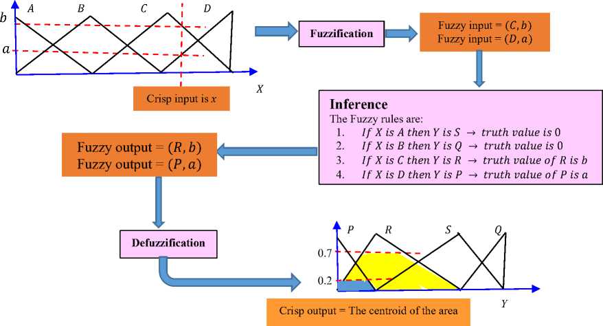
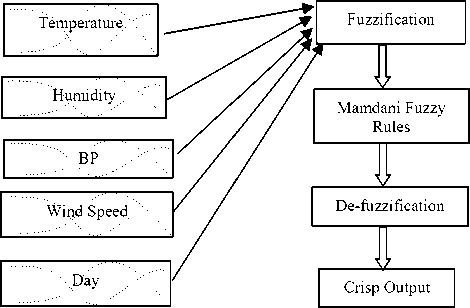
Fig.1. Basic building block of FIS

• 3.1.    Mamdani FIS

• 3.2.    FCM

The numerical data against any independent variable in real life is called crisp value. For a FIS (fuzzy inference system) the numerical data is converted to linguistic value associated with a linguistic variable. This conversion is called fuzzification of crisp value. The input fuzzy variables and output fuzzy variables are related using fuzzy inference rules. Next, the output fuzzy values are again converted to crisp value using de-fuzzification techniques. There are several types of de-fuzzification in FIS like: centroid method, bisector method, Middle of Maxima etc. The entire operation of FIS is found in [19-21]. The basic building block of FIS is shown in Fig.1, where X is the input base variable having four fuzzy values: A, В, C and D. The output base variable Y also has four fuzzy values: P, R, S and Q. The crisp value x provides two fuzzy values (C,b) and (D,a), which again produces two output fuzzy values: (R,b and (P, a) from the rules of inference block. Finally, the defuzzification block evaluates the output crisp value from centroid of the intersected area of output membership functions.

The FCM is an unsupervised learning, which segregate data points based on their internal characteristics. Consider a set of points pt = (xi,yt); i = 1,2,3,. ,n and a set of cluster with centre Cj, j = 1,2,3,... ,k. The probability that a point pm to be under the rth cluster whose centre is Cr, P(pm 6 Cluster — r) = pmr, which is known as the grade of MF of mth point pm under the rth cluster. With each iteration the centre of a cluster Cj and grade of MF of each point against each cluster is updated till the variation of centre and MFs fall below the threshold value found in [22,23].

The basic steps of FCM algorithm are given below.

For input, Data points p i = (x ^ ,y t ), i = 1,2,3, ...,N

Number of cluster c,

The MF matrix , p(b) =

■ p11 p12 p13 •   p1C~ p21 p22 p23 •   p2C .pN1 pN2 pN3 ’   pNc. such that Xk=1pik = 1

In output data points under corresponding cluster

Z^)^ ^(^Л

Step-1 Determine centroid of each cluster using, C j = I —_N .   ._m , —n r  \^m ), j = 1, 2, 3,—, c

Z iNl ljU j )      ^ iN1 ⁽ ^ ij )

Step-2 Update the truth value of MF using, p_t j = ------------—, m>1 is an integer.

_yc (h^-^^-1

^{L k} = ¹ [ iv_l-c _k ^ }

Step-3 Repeat step 1 and 2 until change in objective function,/m = XiL1XC=1(pij)m \\pt — Cj^ is less than a threshold.

• 3.3.    Takagi-Sugeno model

Consider two input variables x and y (linguistic variable) applied in a FIS having two fuzzy sets A and B. The basic format of fuzzy rule under Takagi-Sugeno model is,

If x is A and y is B then output w = f(x,y).

Consider the belonging of x under a fuzzy set A 1 is p_Ai (x") and that of under A ₂ is p_A^ (x). Similarly, the belonging of y under a fuzzy set B 1 is p_B1(y') and that of under B ₂ is p_B2(y)Now two fuzzy rules of Takagi-Sugeno can be expressed as,

If x is A1 and y is В1 then output w1 = f1(x,y') = a-x + b-y +c

If x is A2 and y is B2 then output w2 = f2 (x, y) = a2x + b2y +c

Where a 1 , b 1 , a₂, b₂, c 1 , and c₂ are constant.

Considering numerical value of input variables, x = x₀ and y = y₀. Now, the weighting factor of Takagi-Sugeno model in generalized form is, a t = y_A.(x₀) Л p_Bi(y₀).

a-= BA1(xo)^PBi(yo) = min(pA1(xo),PB1(yo))(1)

a2 = BA2(xo)ApB2(yo) = min(pA2(xo),BB2(yo))(2)

The MFs of fuzzy sets are shown in [24,25].

The final crisp output will be,

Wo

_ a i f i (X o ,y o )+a 2 f 2 (X o ,y o )

a 1 +a₂

The complexity of defuzzification of Mamdani FIS is eliminated in Takagi-Sugeno model found in [26,27].

• 3.4.    ANFIS

4.    Methodology

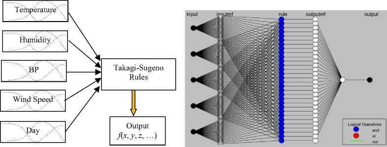
An ‘adaptive neuro-fuzzy inference system’ or ANFIS is a combination of fuzzy inference system and artificial neural network (ANN), takes the advantages of both systems. Here TSK is taken as the fuzzy inference system. The ANFIS has of five layers namely: fuzzy layer, product layer, normalized layer, de-fuzzy layer, and total output layer explained in [28,29]. The most simplified diagram of ANFIS is shown in Fig.2. The square blocks of first layer provides the grade of MF of the base variable x against the fuzzy values A 1 and A 2 . It also gives the grade of MF of the base variable y against the fuzzy values B 1 and B₂. The circular nodes of second layer multiplies the incoming signals like: ^wi = B_Ai(x) B_Bl(y), i = 1, 2 called the firing strength of a rule. The third layers normalize the firing strength like, W i = — +^ , i = 1, 2. The output of fourth layer is, W i .f i , where f_i = a_ix + biy + c_i, i=1,2. The final output is, £ 2=1 W_i. f i , The coefficients {a i , b i , c_i} are adjustable to change final output of the ANFIS.

x

y

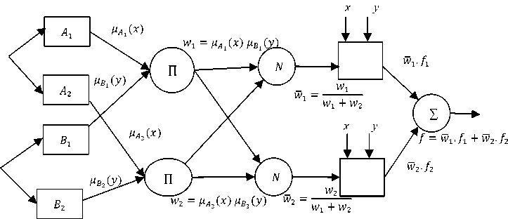
Fig.2. Basic structure of ANFIS

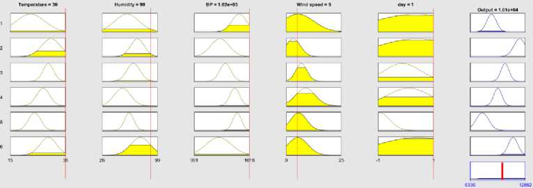
In this paper, the short-term electrical load forecasting is implemented by three different approaches under Matlab 18. The methods are: (i) direct application of crisp data to Mamdani FIS (ii) application of crisp data set to Takagi-Sugeno model (iii) classify data using FCM then apply the classified data to Mamdani FIS (iv) using ANFIS. The output of four techniques is compared to choose the best one. The Fuzzy system used in this research work under the quintuple: ( X , T ( X ), U , G , M ) is shown in Fig.3 like [30,31]. Here, X indicates the base variable, T ( X ) means linguistic value, U refers to linguistic variable, G defines the syntax rule and M is responsible for semantic rule. The operation of Mamdani FIS, Takagi-Sugeno FIS and FCM+FIS are given by the algorithms: 1, 2 and 3 respectively.

Algorithm-1

• •    Read crisp data in tabular form where attributes are the fuzzy variable.

• •    Convert the crisp value in the linguistic value.

• •    From the Table of linguistic value derive possible fuzzy rules.

• •    Considering the range of crisp value of each attribute, design the MF against for each Fuzzy variable.

• •    Applying fuzzy values along with fuzzy rules to the FIS (Fuzzy Inference System).

• •    Design appropriate membership function (MF) of fuzzy output variable (load demand)

• •    De-fuzzified the output Fuzzy values (Linguistic value) to crisp value.

• •    Test the input data vector and evaluate percentage of error.

Algorithm-2

• •    Read crisp data in tabular form.

• •    Considering the range of crisp value of each attribute, design the MF against for each Fuzzy variable.

• •    Apply Takagi-Sugeno rules to relate input variables with the crisp output.

• •    Test the input data vector and evaluate percentage of error.

Algorithm-3

• •    Read crisp data in tabular form where attributes are the fuzzy variable.

• •    Apply FCM to make data clustering.

• •    Repeat step- 2 to 8 of Algorithm-1

5.    Results and Discussions

The complete data flow mode the paper is shown in Fig.4, where four results are compared. In this paper we also used Multiple Linear Regression (MLR) of [32,33] to predict output. MLR is only for comparison with four MLs of the paper. Next section provides results based on analysis of this section.

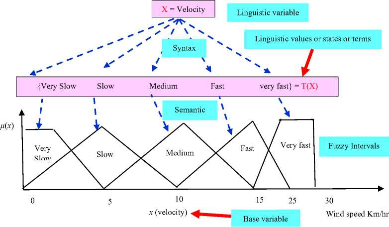
Fig.3. Syntax and semantics in fuzzy system

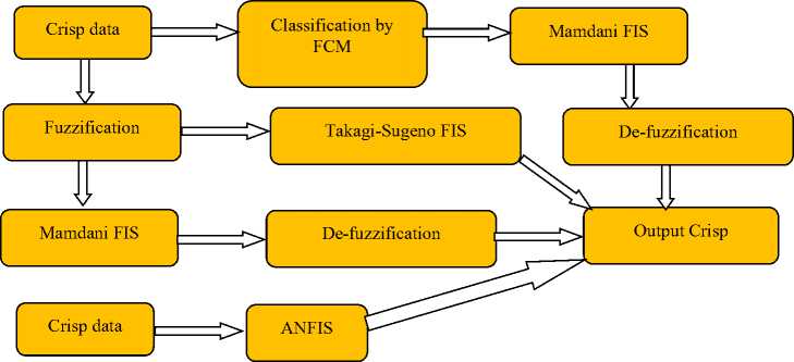
Fig.4. Data flow model

We take daily load and weather parameters from BPDB and ‘Accuweather’ website to train the ML models. The weather and load data of a year is used to train the model, but more data can be used (for example last ten years data) to train the ML model to get more accurate results. First of all, we applied Multiple Linear Regression like [34-36] on the entire dataset and found low correlation between inputs attributes and output load visualized from Fig. 5. Although the mean error is found 6.3228% but some points provide error, more than 20%. Therefore, segment wise approach i.e. FIS is more realistic for this analysis to reduce both mean and instantaneous error.

Next, we use FIS of Takagi-Sugeno method like Fig. 6(a) found in [37], where input and output is related by linear equation like: IF x is A and у is В THEN Z = f(x,y). The structure of corresponding ANFIS found from Matlab 18 is shown in Fig. 6(b) with 30 possible output levels. The linear relationship between five input variables and i^th output is expressed as, y_t = a , x temperature + b_tx Humidity + c_tx ВР + d_tx Wind_speed + e_tx day + f t - For example the six coefficients for output y 1 is found as: [69.66 -21.87 -65.56 -100.9 0 7.524e+04] and that of 29 ^th output y₂₉ is [1746 -516.9 1468 -3347 -1.485e+06 0]. The dynamic Takagi-Sugeno model takes the MFs of variables like Fig. 7. In this model we got 30 Fuzzy rules shown in Fig. 8. This type of set of rules are used as the knowledge bank of an expert system like [38]. The variation of fuzzy input variables against output is shown in Fig. 9 as the surface plot.

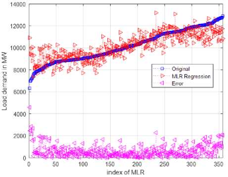
Fig.5. MLR output of load forecasting

(a) FIS model                             (b) ANFIS model

Fig.6. Basic of takagi-sugeno

Air Pressure

Humidity

Wind Speed

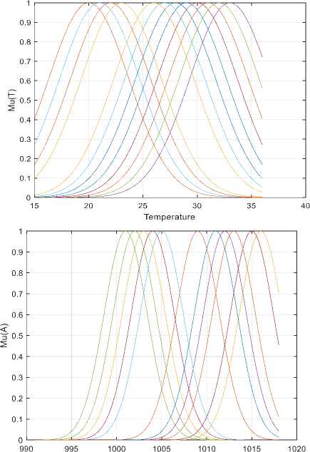
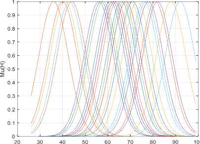
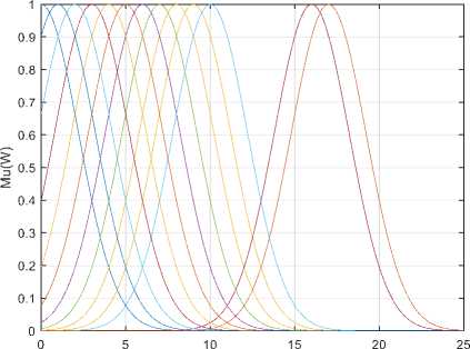
Fig.7. MFs of linguistic variables

1 К (Temperature is inldusterl) and (Humidity is m2duster1) and (BP is in3duster1) and (Wind speed is in4cluster1) and (day is inbdusterl) then (Output is out 1 cluster 1) (1) 2 If (Temperature is in1cluster2) and (Humidity is in2duster2) and (BP is in3duster2) and (Wind speed is in4cluster2) and (day is inSckrster?) then (Output is out1 clusters) (1} 3 If (Temperature is in1 cluster!) and (Humidity is in2cluster3) and (BP is in3duster3) and (Wind speed is in4cluster3) and (day is in5cluster3) then (Output is out1 cluster!) (1) 4 If (Temperature is inldusterf) and (Humidity is in2duster4) and (BP is in3duster4) and (Wind speed is in4cluster4) and (day is in5ctuster4) then (Output is out1cluster4) (1) 5 If (Temperature is in1duster5) and (Humidity is in2duster5) and (BP is in3cluster5) and (Wind speed is in4cluster5) and (day is in5cfuster5) then (Output is out 1 clusters) (1) 6 It (Temperature is inldustefB) and (Humidity is inZdustetf) and (BP is in3cluster6) and (Wind speed is in4duster6) and (day is in5ctuster6) then (Output is out1cluster6) (1) 7 If (Temperature is inldusterT) and (Humidity is in2cluster7) and (BP is in3cluster7) and (Wind speed is in4cluster7) and (day is in5cfuster?) then (Output is out1 cluster?) (1) 8 If (Temperature is In1duster8) and (Humidity is in2duster8) and (BP is in3duster8) and (Wind speed is in4cluster8) and (day is in5cluster8) then (Output is out 1 clusters) (1) 9 If (Temperature is in1duster9) and (Humidity is in2clustec9) and (BP is in3duster9) and (Wind speed is in4cluster9) and (day is in5cluster9) then (Output is outlclusterB) (1) 10 If (Temperature is in1 dusteMO) and (Humidity is in2clusten0) and (BP is in3cluster10} and (Wind speed is in4duster10) and (day is in5cluste<10) then (Output is out 1 clusterl 0} (1) 11. If (Temperature is in1 ousted 1) and (Humidity is in2clusteri 1) and (BP is in3cluster11) and (Wind speed is In4duster11) and (day is inScluster 11) then (Output is out1cluster11) (1} 12 If (Temperature is inf clusterl 2) and (Humidity is in2cluster12) and (BP is in3cluster12) and (Wind speed is in4cluster12)and (day is in5cluster12) then (Output is out 1 cluster 12) (1) 13 If (Temperature is in1c!uster13) and (Humidity isin2cluster13)and (BP is In3clusler13)and (Wind speed is In4cluster13)and (day tsin5cluste<13) then {Output is out 1 cluster 13}(1)

14 If (Temperature is ml cluster 14) and (Humidity isin2clusterl4) and (BP is in3cluster14)and (Wind speed is in4cluster14)and (day ism5cluster14) then (Output is outlcluster 14) (1) 15 If (Temperature is in1 clusterl 5) and (Humidity is in2clustert5) and (BP is in3cluster15) and (Wind speed is in4cluster15) and (day is in5cluster15) then (Output is out 1 cluster 15) (1) 16 If (Temperature is inf clusterl 6} and (Humidity is in2cluster16) and (BP is in3cluster16) and {Wind speed is in4cluster16) and (day is in5cluster16) then (Output is out 1 cluster 16) (1) 17 If (Temperature is inldusterl?) and (Humidity is in2ctuster17) and (BP is in3cluster17) and (Wind speed is iMdusterl 7) and (day is inSclusterl 7) then (Output is out!clusterl7) (1)

18 If (Temperature is in1cluster18) and (Humidity is in2cluster18) and (BP is in3clustei 18) and (Wind speed is in4duster18) and (day is in5cluster18) then (Output is out!clusterl8) (1) 19 II (Temperature is inlclustei 19) and {Humidity is in2duster 19) and (BP is m3cluster19) and (Wind speed is in4duster19) and (day is in5cluster19)then (Output is outlcluster 19) (1) 20 If (Temperature is in1cluster20) and {Humidity is in2ciuster20) and (BP is in3cluster20) and (Wind speed is in4ciuster20) and (day is in5cluster20) then (Output is aut1cluster20) (1) 21 If (Temperature is in1duster21) and (Humidity is in2ctuster21) and (BP is in3cluster21) and (Wind speed is in4duster21) and (day is in5duster21) then (Output is outlduster21) (1) 22 If (Temperature is in1duster22) and {Humidity is In2ciuster22) and (BP is in3clusler22) and (Wind speed is in4duster22) and (day is in5cluster22) then (Output is out1cluster22) (1) 23 If (Temperature is n1cluster23) and (Humidity is in2duster23) and (BP is in3duster23) and (Wind speed is in4duster23) and (day is in5duster23) then (Output is out1clister23) (1) 24 If (Temperature is rn1duster24) and (Humidity is in2duster24) and (BP is in3duster24) and (Wind speed is in4duster24) and (day is in5duster24) then (Output is out1duster24) (1) 25 If (Temperature is in1duster25) and (Humidity is in2duster25) and (BP is in3duster25) and (Wind speed is in4duster25) and (day is in5duster25)then (Output is out1duster25) (1) 26 If (Temperature is m1duster26j and (Humidity is in2ctuster26) and (BP is in3duster26| and (Wind speed is in4duster26) and (day is in5duster26) then (Output is out1duster26) (1) 27 If (Temperature is m1cluster27) and (Humidity is in2ctuster27)and (BP is in3duster27) and (Wind speed is in4duster27) and (day is in5dustei27) then (Output is out1duster27) (1) 28 If (Temperature is m1duster28) and (Humidity is in2ctuster28) and (BP is in3cluster28) and (Wind speed is in4ciuster28) and (day is in5duster28) then (Output is out1cluster28) (1) 29 If (Temperature is in1cluster29) and (Humidity is in2cluster29) and (BP is in3cluster29) and (Wind speed is in4cluster29) and (day is in5ciuster29) then (Output is out1cluster29) (1) 30 If (Temperature is in1duster30) and {Humidity is in2ctuster30) and (BP is in3cluster30) and (Wind speed is in4ciuster30) and (day is in5duster30) then (Output is out1cluster30) (1)

Fig.8. Fuzzy rules

Fig.9. Surface plot of Fuzzy input variables under Takagi-Sugeno

Next, we applied Mamdani rules on FIS as shown in Fig. 10, where both the input and output variables have several levels (2 to 5 levels). In this paper we used 225 fuzzy rules on the Mamdani FIS and few of them are shown in Fig. 11. The variation of fuzzy input variables against output for Mamdani FIS is shown in Fig. 12 as the surface plot. The similar plot is shown for FCM + Mamdani in Fig. 13.

• •    If (temperature is High) and If (Humidity is Very High) and If (Pressure is Medium) and If (Wind speed is Medium) and If (Day is Normal) then (Generation is High)

• •    If (temperature is Very High) and If (Humidity is High) and If (Pressure is Medium) and If (Wind speed is Medium.) and If (Day is Normal) then (Generation is Very High)

• •    If (temperature is High) and If (Humidity is Medium) and If (Pressure is Medium) and If (Wind speed is Medium) and If (Day is Normal) then (Generation is High)

• •    If (temperature is Medium) and If (Humidity is High) and If (Pressme is Very High) and If (Wind speed is Medium) and If (Day is Normal) then (Generation is Medium)

• •    If (temperature is Low) and If (Humidity is Medium) and If (Pressure is Very High) and If (Wind speed is Medium) and If (Day is Normal)

then (Generation is Medium)

• •    If (temperature is Medhun) and If (Humidity is Medium) and If (Pressure is Very High) and If (Wind speed is Medium) and If (Day is Normal) then (Generation is Medhun)

• •    If (temperature is High) and If (Humidity is High) and If (Pressure is Medhun) and If (Wind speed is Medhun) and If (Day is Holyday) then (Generation is Low)

• •    If (temperature is Medimn) and If (Humidity is High) and If (Pressure is High) and If (Wind speed is Medhun) and If (Day is Holyday) then (Generation is Low)

• •    If (temperature is High) and If (Humidity is Medimn) and If (Pressure is High) and If (Wind speed is Slow) and If (Day is Holyday) then (Generation is Low)

• •    If (temperahire is Medium) and If (Humidity is High) and If (Pressure is Very High) and If (Wind speed is Medimn) and If (Day is Holy day) then (Generation is Low)

Fig.11. Few fuzzy rules of Mamdani FIS

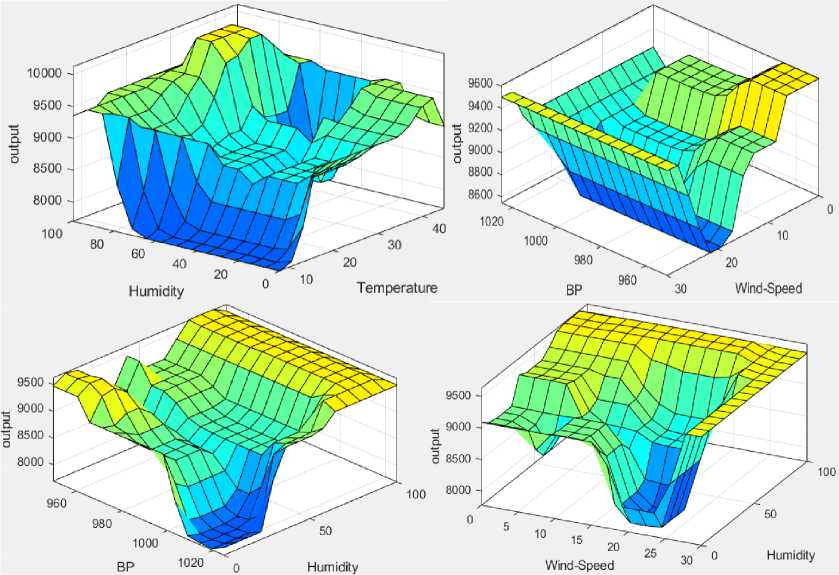
Fig.12. Surface plot of fuzzy variables under Mamdani FIS

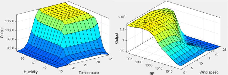
Fig.13. Surface plot of Fuzzy variables under FCM + Mamdani FIS

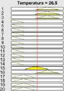
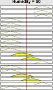
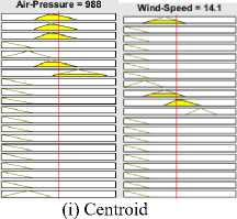
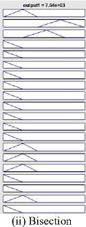
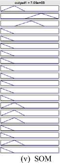
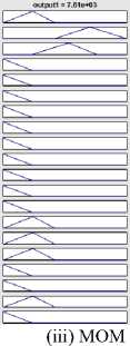
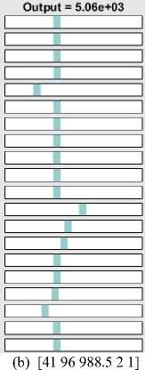
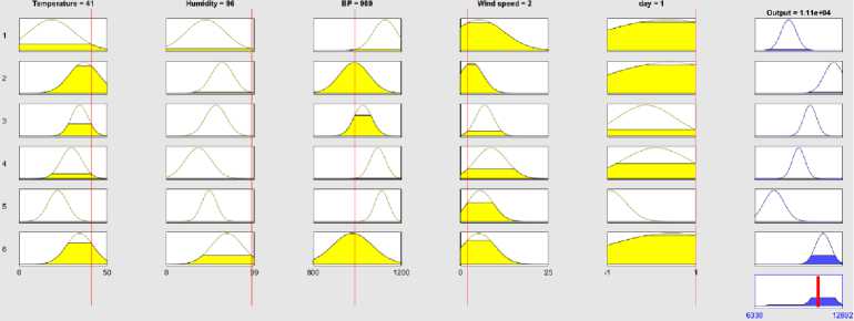
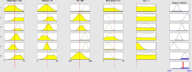
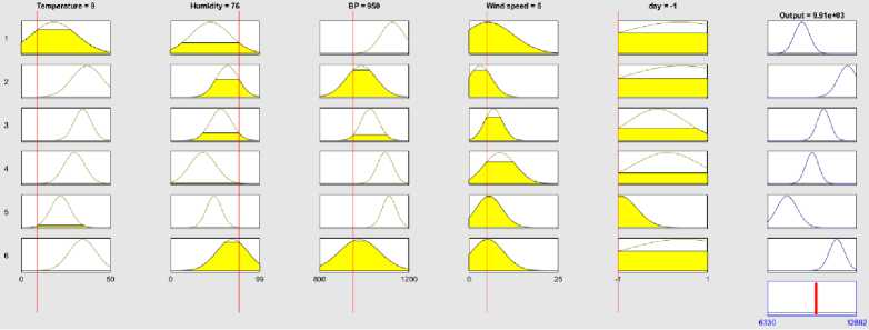
The verification of test data on fuzzy rules under Mamdani FIS are shown in Fig. 14(a)-(d) for four test vectors [Temperature Humidity Air Pressure Wind-Speed Day] as [36 90 1025 5 1], [41 96 988.5 2 1], [26.5 50 988 14.1 -1] and [9 76 950 5 -1]. The first vector is for hot and humid day, the second vector is for very hot and humid summer day, the third one for moderate weather and the fourth one is for dry cool weather. The Mumdani test is done against four defuzzification techniques: Centroid, Bisection,MOM, IOM and SOM. The output of Takagi-Sugeno FIS for the same test vector set are shown in Fig. 15(a)-(d) and provides the closed results like Mamdani FIS. Similar test results are shown in Fig. 16(a)-(d) for FCM + Mamdani FIS.

Centroid, Bisection, MOM, IOM and SOM

(a) Test = [36 90 1025 5 1]

(i) Centroid

(ii) Bisector

(iii) MOM

(b) Test = [41 96 988.5 2 1]

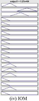
Table 2. Takagi-sugeno FIS

Temperature	Humidity	Air pressure	Wind	Day	Load Demand	FIS	% error
(°C)		(pa)	(km/h)		(MW)
28	84	1007	3	-1	10988	11200	1.93
26	94	1004	5	-1	10262	10300	0.37
27	66	1014	2	-1	9242	8980	2.83
29	78	1004	1	1	12317	12100	1.76
34	67	998	1	1	12220	12300	0.65
19	62	1014	7	1	8584	8800	2.51
Average							1.675

(c) Test = [26.5 50 988 14.1 -1]

(i) Centroid

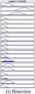
Fig.14. Verification of test data under Mamdani FIS

(v) SOM

(d) Test = [9 76 950 5 -1]

The percentage of deviation of practical output and Takagi-Sugeno is shown in Table 2. Three de-fuzzification techniques: Centroid, Bisection and MOM are shown in Table 3 for Mamdani FIS. The same result is shown in Table 4 for FCM+Mamdani.

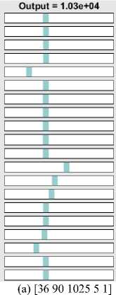
Fig.15. Output of Takagi-Sugeno FIS for the same test vector

(a) [36 90 1025 5 1]

(b) [41 96 988.5 2 1]

(c) [26.5 50 988 14.1 -1]

(d) [9 76 950 5 -1]

Fig.16. Output of FCM + Mamdani for the same test vector

Table 3. FIS under Mamdani

Load Demand (MW)	FIS (Centroid)	% error (Centroid)	FIS (Bisector)	% error (Bisector)	FIS (MOM)	% error (MOM
10988	10900	0.801	10900	0.80	10900	0.80
10262	10450	1.83	10600	3.29	10900	6.22
9242	9550	3.33	9600	3.87	9680	4.74
12317	12100	1.37	11900	3.38	11900	3.38
12220	11900	2.61	11600	5.07	11600	5.07
8584	8450	1.56	9100	6.01	9200	7.17
Average		1.91		3.74		4.56

Table 4. FIS under FCM +Mamdani

Load Demand (MW)	FIS (Centroid)	% error (Centroid)	FIS(Bisector)	% error (Bisector)	FIS (MOM)	% error (MOM)
10988	11100	1.02	11300	2.83	11400	3.75
10262	10400	1.34	11100	8.16	10400	1.34
9242	9540	3.22	9700	4.95	9820	6.25
12317	12300	2.29	11400	7.44	11400	7.45
12220	12500	2.29	11700	4.25	12200	0.16
8584	9030	5.19	9060	5.54	9340	8.01
Average		2.56		5.53		4.49

Finally, the entire dataset is applied on an ANFIS to train it. The profile of training data and the output of ANFIS with error is shown in Fig. 17. Using 357 data records the mean percentage of error is found 3.62%.

-Training Data - ANFIS Output

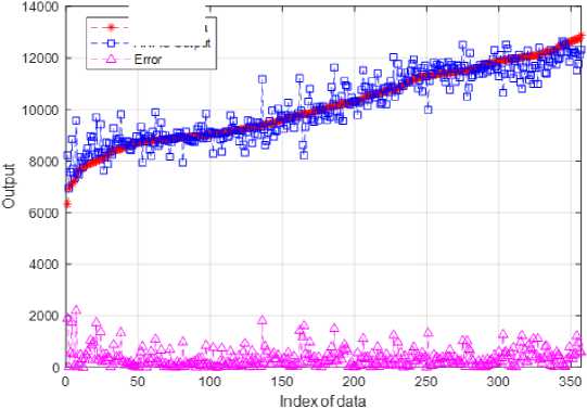
Fig.17. Profile of training and ANFIS output

The average percentage of error was found 1.675% for Takagi-Sugeno, 1.91% for Mamdani and 2.56% for FCM + Mamdani from Table 2 to 4. The ANFIS model taking all the five fuzzy variables provides the error of 3.62%. In [39] four input fuzzy variables: temperature, humidity, season and peak hour are considered under FIS and average percentage of error was found higher than this paper again, also few records show the percentage of error greater than 12%. In [40] authors used ‘date type’, ‘daily mean temperatures’ and ‘electric load data’ as the parameters of ANFIS. Few pints on the graph of ‘forecast value’ and ‘aimed value’ shows wide separation because of using only three parameters. This paper shows smoother results compare to [40] because of use of five input fuzzy variables and five linguistic values against each variable. Four variables: seasons, weekly day, daylight hours and temperature were used as the input in [41] and the historical electric load is taken as the target under ANFIS model. The percentage of error was found above 8% because of exclusion of two vital weather parameter: humidity and wind speed of this paper. The results of four techniques used in this paper is found better than above three previous works.

6.    Conclusions and Future Works

We develop short term electrical load forecasting model using four types of FIS where three types of defuzzifications are applied under Mamdani FIS to test the accuracy of predicted load. Compared to previous research works, more fuzzy variables and fuzzy values are considered in this paper hence it can be considered as the most details fuzzy based load forecasting model. In any fuzzy inference system output accuracy improves with incorporation of more fuzzy values under each fuzzy variable. Even incorporation of more fuzzy variables will also improve accuracy. For both the cases, number of fuzzy rules and computational complexity will be increased. In future we will add some other variables like ‘Rainy day’, ‘hot and humidity day’, ‘peak season of irrigation’, ‘religious occasion like Ramadan’ etc. to enhance accurate prediction of load at the expense of process time. We also have the scope to apply back propagation algorithm of ANN, Long Short Term Memory (LSTM) and convolutional neural network (CNN) of deep learning to relate the weather parameters with the actual electrical load for comparison.

Acknowledgment

We are grateful to the NST Fellowship under Ministry of Science and Technology, Bangladesh for funding the research work of this paper.