Simplified real-, complex-, and quaternion-valued neuro-fuzzy learning algorithms

Published Online May 2018 in MECS DOI: 10.5815/ijisa.2018.05.01

Neuro-fuzzy methods refer to combinations of artificial neural networks and fuzzy models [1-3]. Artificial neural networks are the computational models of neuronal cell behaviors in the brain, and have high learning ability as well as parallel processing ability. These properties allow systems to perform well in environments that are difficult to formulate. Fuzzy logic is based on inference rules and allows the systems to use human-like “fuzziness.” In particular, fuzzy inference systems based on if–then rules provide high robustness and human-like inference [4, 5]. However, it is usually hard for human being to design proper fuzzy rules resulting the consumption of a considerable time to tune fuzzy rules. Neuro-fuzzy methods having learning algorithms of artificial neural networks in the fuzzy inference systems can solve these problems. Conceiving complementary strengths of neural and fuzzy systems, neuro-fuzzes have been applied to handle numerous real-life problems including control, function approximations, classifications, etc. [1-3, 6-8].

A variety of system structures and learning algorithms are available for neuro-fuzzy methods [9–26]. Learning of the classical neuro-fuzzy systems is based on the gradient descent method [9]. It is modified to avoid non-firing or weak firing [10, 11] and to improve learning efficiency [12]. Genetic algorithms are applied to a neuro-fuzzy with radial-basis-function-based membership for the automatic generation of fuzzy rules [13]. An adaptive neuro-fuzzy system for building and optimizing fuzzy models has been proposed [14]. A variety of neuro-fuzzy methods are also proposed recently [15–21]. The applications of neuro-fuzzy methods include feature selection [19, 21], classification [15–20], and image processing [17]. Furthermore, neuro-fuzzy methods using complex-valued inputs and outputs have been proposed and applied to image processing and time-series prediction [22, 23]. In addition, recent studies of neuro-fuzzy methods heaving complex-valued or quaternion-valued inputs and realvalued outputs exhibit better learning ability than the conventional methods [24-28].

The conventional real-valued neuro-fuzzy method (RNF) is based on classic fuzzy systems with antecedent membership functions and consequent singletons. When training data with input-output mapping are given to the network, the membership functions and singletons are tuned by back propagation algorithm. However, the number of fuzzy rules rapidly increases with the increment of the number of inputs. In the RNF, the number of fuzzy rules is calculated by the number of inputs to the power of the number of divisions of input space; hence, the learning time increases with inputs.

RNF extensions in complex and quaternion domains reduce the network parameters of a given problem with a less number of inputs. Complex-valued neuro-fuzzy method (CVNF) has complex-valued fuzzy rules whose inputs, membership functions, and singletons are complex numbers, and outputs are real numbers. On the other hand, quaternion neuro-fuzzy method (QNF) has quaternionvalued fuzzy rules whose inputs, membership functions, and singletons are quaternions, and outputs are real numbers. Different individual activation functions are investigated to get real-valued outputs from complexvalued net-input and quaternion-valued net-input in CVNF and QNF, respectively. The network parameters of CVNF and QNF are tuned by complex-valued and quaternion-based back propagation algorithms, respectively [24-28].

The CVNF can treat two real-valued inputs as one complex-valued input, and the QNF can treat four realvalued inputs as one quaternion-valued input. Thus, when RNF, CVNF, and QNF are applied to the same problem, CVNF and QNF have fewer network parameters than RNF. CVNF and QNF have also shown better learning abilities for function approximations and classifications due to less variables. In the function approximations, CVNF has identified some nonlinear functions better than RNF [24, 25]. In classifications, QNF has shown better classification abilities than RNF [27]. Nevertheless, both CVNF and QNF still have the problem of rapidly increasing number of parameters when the number of inputs increases.

This study investigates simplified fuzzy rules that constrain rapid increment of rules with inputs; and proposed simplified RNF (SRNF), simplified CVNF (SCVNF) and simplified QNF (SQNF) employing the proposed simplified fuzzy method in conventional methods. The proposed SRNF, SCVNF, and SQNF are new neuro-fuzzy learning methods that differ from the conventional methods in their fuzzy rule structures. These new methods have simplified the fuzzy rules, and tuned the fuzzy rules based on the gradient descent method. In these methods, the number of rules are equal to the number of divisions of input space and independent of the number of inputs. Thus, the proposed methods can constrain the rapid increment of parameters, even when the number of inputs increases. Simulations that compare the new methods with the conventional methods show that the new methods have the same learning abilities as the conventional methods.

The remainder of this paper is structured as follows. Section II discusses the conventional methods, RNF, CVNF, and QNF. Section III demonstrates the proposed simplified methods, SRNF, SCVNF, and SQNF. Section IV compares the proposed methods with the conventional methods on function approximation problems. Section V shows the performances of the proposed methods on real-world benchmark problems for supervised learning with continuous and discrete outputs. Finally, Section VI concludes the paper with a discussion as well as possible future researches based on current study.

• II.    Conventional Neuro-Fuzzy Methods

Conventional methods include RNF, CVNF, and QNF. To make the paper self-contained as well as for better understanding of the proposed methods, following subsections describe each of these conventional methods in sequence.

• A.    Real-Valued Neuro-Fuzzy Method (RNF)

RNF tunes antecedent membership functions and consequent singletons of the fuzzy rule by the gradient descent method. This method is based on the if–then rule of fuzzy inference. For example, let the input to be x_p (р = 1,2) and the output to be y , and each input space is divided by three membership functions, then the fuzzy inference rules are given as follows.

Rule 1: If x1 is A11 and x2 is A12, then у is w1

Rule 2: If x1 is A21 and x2 is A22, then у is w2

Rule 9: If x1 is A91 and x2 is A92, then у is w9

Here, A_qp(q = 1,2,•••,9; р = 1,2) are antecedent membership functions and w_q(q = 1, 2, •, 9) are consequent singletons for each rule.

Fig. 1 illustrates the conventional RNF of the system with two inputs and one output. Each input space is divided into three; therefore, three membership functions are required for each space to generate the antecedent grades. The gravity method is applied to generate the output. The total number of membership functions is 32x2=18 (AH,™,A92), and the number of antecedent grades is 32=9 (h1, ™,h9) which is equal to the number of rules. The number of parameters to be determined is 18×2+9=45. In this case, Rule 1 uses the first membership functions of both x1 and x2. Rule 2 uses the first membership function of x1 and the second one of x2. Rule 9 uses the third membership functions of both x1 and x2 . The rules are made by all combinations of membership functions for each input. Thus, the number of fuzzy rules depends on the number of divisions of each input space. The total number of rules is the number of divisions of each input space to the power of the number of inputs (i. e., (rules) = (divisions)(mp“£s:)).

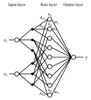
Fig.1. Conventional RNF with two inputs and one output where each input space is divided into three.

Signal flow in this case is as follows. First, when inputs enter the network, each input (i.e., x p ) passes through the antecedent membership function corresponding to the fuzzy rules. The membership functions A_qp are given by a Gaussian function as

A qp = exp{- (

,^xp d qp ^b qp

£},

where aqp and bqp are respectively the center and width of the function. Second, in each rule layer node, the antecedent grade hq(q = 1,2, —,9) for the fuzzy rule is calculated by the algebraic product of membership functions as hq =Пр=1 Aqp .               (2)

Then, at the output node, the inference result y is given by the gravity method with the antecedent grade h_q and consequent singleton w_q :

У =

X q=1 b q ^w q

X q=1 ^b q

The above signal flow is the same as that of the classic fuzzy inference method with the if-then rule. RNF tunes each of the network parameters by back propagation algorithm. If the desired output to be t „ (n = 1,2, — ,^) and the current output to be y „ , then the error function to be minimized during training is given by

E = | Z "=i (t „ -y „ )². (4)

During training, the network parameters w_q,a_qp,b_qp are updated by

£-a/,(5)

„ ар

£a„.       P.     ,(6)

dp

-'^       у..,.(7)

where a, P, and у are the respective learning rates. The learning process can be performed by giving an initial value to each of the network parameters and iterating Eqs. (5)–(7). In the RNF, each antecedent membership function of input spaces corresponds independently to each fuzzy rules. Thus, the network has high degree of freedom, and can fit well the training data [9].

• B.    Complex-Valued Neuro-Fuzzy Method (CVNF)

CVNF is an extension of RNF to complex numbers [24, 25]. The inputs, antecedent membership functions, and consequent singletons are in complex domain whereas output is real. Like RNF, the network is composed of input, rule, and output layers. In the network, a complex value based on a specific rule called the “complex fuzzy rule” is passed through the activation function to output the real value. For example, let the complex-valued input to be x_p = x R + i^ P (p = 1,2) and the complex-valued net-input of the output node to be z = z^R + iz¹ , then the fuzzy inference rules are given as follows. Superscripts R and I denote the real and imaginary parts of complex numbers. Further, i refers to the imaginary part of a complex number.

Rule 1: If x1 is A11 and x2 is A12, then zis

Rule 2: If x1 is A21 and x2 is A22, then zis w

Rule 9: If x1 is A91 and x2 is A92, then zis w

Here,  Aqp = ARp + iAqp is the  complex-valued antecedent membership function and wq = wRR +i^q is the complex-valued consequent singleton.

First, inputs pass through the antecedent membership functions corresponding to the fuzzy rules

A. exp' \-  ',           (8)

where C = R or 7 . The Gaussian functions are independently assigned to the real and imaginary parts of the antecedent membership functions. CVNF can thus generate the real and imaginary parts of complex-valued membership functions. Here, aqp and bqp are the centers and widths, respectively. At each node of the rule layer, the real and imaginary parts of the complex-valued antecedent grades hq are calculated as hq = np=1A^p .                 (9)

Then, at the output node, the complex-valued net-input z is given by the same term as the gravity method Eq. (3), but the parameters are complex values.

^iM+^M+iwq) ^ q=1 (^ q ^{+ik q )}

Finally, the activation function fc^R(x) converts the complex-valued net-input z to the real-valued inference result y as y = fc^R(z) , (11)

f^z) (M<) M/)f , (12)

where fR(x) = 1/(1 + e-3z). Eq. (12) is considered in recent studies of complex-valued neural networks [30, 31].

The error function has the same formula as of RNF in Eq. (4). During training, the parameters w_q,a_qp,b_qp are updated by

Awq =-a^o - ia^y,(13)

q        awR      awq’

.                ан.ан

^аqP = -P-^R-- il^, auqp

Д^ = -У5--1У5-.(15)

^aa qp       ^aa qp

The learning process can be performed by giving an initial value to each parameter and iterating Eqs. (13)– (15).

In CVNF, two real-valued inputs can be used as one complex-valued input. Thus, CVNF has fewer parameters than RNF when both are applied to the same problem. The number of parameters in the complex-valued methods can be obtained by

(parameters') =

(inp'uts) x (rules) x 2 # ¹ + (singletons) # ²

• #1: (centers and width of membership function)

#2: (singletons) = (rules)           (16)

Here, in case of complex-valued methods, the number of parameters is twice the number of parameters as mentioned in Eq. (16), while the number of inputs becomes half.

For example, the problem of Fig. 1 heaving two realvalued inputs and one output, the number of input nodes in RNF is two, and in CVNF that is one. Then, the number of rule nodes in CVNF is 3¹ = 3 as of three functions for each input space, while the number of rule nodes in RNF is 3² = 9 . In this case, the number of network parameters in CVNF is (1 x 3¹ x 2 + 3¹) x 2 = 18 while the number is 45 (= 2 x 3² x 2 + 3²) in RNF. In comparisons of both methods by function identifications, the CVNF showed same or better learning ability than that of RNF. Detailed description of CVNF is available in our previous studies [24, 25].

• C.    Quaternion Neuro-Fuzzy Method (QNF)

QNF is another and recent extension of RNF to the quaternion domain [26–28]. The network has the three-layer structure as that of RNF. Inputs, membership functions, and singletons are quaternion, and the output is real. In the network, signals are processed by quaternion fuzzy rules. If the quaternion-valued inputs are x_p = x R + ix P + jx P + kx R (p = 1, 2) and the quaternionvalued net-input of the output node is z = z^R + iz¹ + jz ^ + kz^K , and there are three divisions of each input space, then the fuzzy inference rules are given as follows.

Rule 1: If x1 is A11 and x2 is A12, then z isw

Rule 2: If x1 is A21 and x2 is A22, then z isw

Rule 9: If x1 is A91 and x2 is A92, then z isw

Here, AOB = A™ + 1Л„„ + jAR„ + kAR„   is the qp qp qp qp qp quaternion-valued antecedent membership function and wq = wR + Vwq + jw^ + kwR is the quaternion-valued consequent singleton. Superscript R denotes the real part, and superscripts I, J, and K denote the imaginary parts. Further, i, j, and k in front of each element of a quaternion number represent unit imaginary numbers with properties i2 = j2 = k2 = ijk = -1.

First, inputs pass through the antecedent membership functions corresponding to the fuzzy rules

''••(                ,            (17)

where Q = R,I,],K (as above). This shows that the membership function is independently set for the real and imaginary parts of the quaternion-valued input. Second, in each rule-layer node, the real and imaginary parts of the quaternion-valued antecedent grades hq are calculated as h-=np=1A-p .             (18)

Then, the net-input z of the output node is given by a gravity-like method:

_ Zq=i (h^R+ih q +jh q +kh ^ )(w^R+iw q +jw ^ +kw ^ ) X q=i (h^R+ ⁱ h q + ^j h q + ^k h^R)

=---------- ⁽ Z ^q = ^ihq w ^q) Cs ^q = ^ihq) ------------ .  (19)

(z q=i< +(z q=i ^k q )^-+(z q=XP (z q=i<

Here, h_q = h R - ih R - jh R - kh R is the conjugate quaternion number of h_q.

Finally, it passes through the activation function, and the real-valued output is generated as v-f,.R(z),             (20)

f_Q ^R (z) = (f R (z^R) - f R (z^;) - f R (z ^ ) - f R (z^R))², (21)

where f_R(x) = 1/(1 + e^-3z). Equation (21) is derived similarly to Eq. (12); the real and imaginary parts of net-input z are separately given to f_R (x) , and then, the difference between the output of real part and the sum of the outputs generated by imaginary parts is calculated and squared.

The error function has the same formula as of RNF in Eq. (4). During training, the parameters wq,aqp,bqp are updated by

^W q

дЕ

—a -—p dw^

—

Va^r dw q

—

ja-^ — ка^к , dw _q       aw q ’

1) Simplified fuzzy rules

In the conventional RNF, signals are processed based on classic fuzzy rules; the rules are constructed in all combinational patterns of membership functions for each input. Thus, an increment of number of inputs causes a rapid increment of the number of parameters, even with a small number of divisions of each input space. To overcome this problem, in SRNF the network processes signals according to rules based on the salient combinations of membership functions. The other combinations are considered to be redundant, and are not used.

^^a qp

—

р^—^^^—^^, (2³)

^da qp

^da qp

^da qp

^bqp =

дЕ

дЕ    . дЕ

■ ^VS& ^— 'V —

^d b ’qp

—

1Г^

^db qp

—

дЕ к.  ■

where a, P, and у are the respective learning rates. The learning process can be performed by giving an initial value to each parameter and iterating Eqs. (22)–(24).

QNF can use four real-valued inputs as one quaternionvalued input, thus reduces the number of parameters compared to CVNF. For example, when a problem has four real-valued inputs and one output, the number of input nodes in CVNF is two, and that in QNF is one. If the number of divisions of each input space is three, then the number of rule nodes in CVNF is 3² = 9, and that in QNF is 3¹ = 3. The number of parameters is quadruple the number of Eq. (16) while the number of inputs becomes one quarter. In this case, the number of network parameters in CVNF is (2 x 3² x 2 + 3²) x 2 = 90, and that in QNF is (1 x 3¹ x 2 + 3¹) x 4 = 36 . Again, for example, if a problem has eight real-valued inputs and one output, and the number of divisions of input space is two, the numbers of input nodes, rule nodes, and total network parameters are 8, 256, and 4352 for RNF; 4, 16, and 288 for CVNF; and 2, 4, and 80 for QNF; respectively.

On function identification and classification problems, QNF showed good convergence and better learning abilities than RNF. Detailed description of QNF is available in our previous studies [26–28].

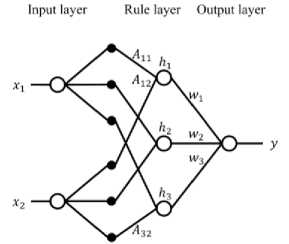
Fig.2. Proposed SRNF with two inputs and one output where each input space is divided into three.

Fig. 2 illustrates the proposed SRNF of the system with two inputs and one output against RNF mechanism shown in Fig. 1. In the SRNF, each input space is divided into three. One membership function is used for each space to generate the antecedent grades. The weighted sum is used to generate the output. If the inputs are x_p (p = 1,2) , the output is y , and there are three divisions of each input space, then the rules are given as follows.

• III.    Simplified Neuro-Fuzzy Methods

This section explains proposed simplified neuro-fuzzy methods. At first, simplified method is explained with RNF and then explains for CVNF and QNF. Finally, proposed simplified methods are demonstrated for a sample problem.

• A. Simplified Real-Valued Neuro-Fuzzy (SRNF)

SRNF is a simplified version of RNF. It differs from RNF in its fuzzy rules and output determination method in output node, but the network structure and signal flow are the same as those of RNF. In the following, two points are explained: 1) simplified fuzzy rules and 2) network calculations.

Rule 1: If x1 is A11 and x2 is A12, then у is и/1 Rule 2: If x1 is A21 and x2 is A22, then у is w2 Rule 3: If x1 is A31 and x2 is A32, then у is w3

Here, Rule 1 uses first membership functions of x 1 and x₂, Rule 2 uses second membership functions of x 1 and x₂, and Rule 3 uses third membership functions of x 1 and x₂. The total number of membership functions is 3x2 = 6 (A 11 , — ,A₃₂), and the number of antecedent grades is 3 (^ 1 , —, h₃) which is equal to the number of rules. The number of parameters to be determined is 6 x 2 + 3 = 15.

Table 1. Number of Parameters for RNF and SRNF on Several Parameter Conditions

Input Divisiona Rule Parameter RNF SRNF RNF SRNF 2 3 9 3 45 15 2 5 25 5 125 25 5 5 3125 5 34375 55 aNumber of divisions of each input space

In this simplified rules, the number of rules is equal to

the number of divisions of each input space ((rules') = (divisions') ). Thus, even if the number of inputs increases, the number of parameters does not increase rapidly. The simplified method can thus be applied to problems with a large number of inputs. Table 1 compares the number of parameters for conventional RNF and the proposed SRNF under several combinations of inputs and divisions. SRNF has fewer parameters than RNF under all conditions.

• 2) Network calculation

In the conventional RNF, the output is calculated by the gravity method at the output node. In contrast, in SRNF the following equation is used instead of the gravity method in Eq. (3):

У = ^ q=1 h q W q . ⁽²⁵⁾

Equation (25) requires that the denominator in Eq. (3) is equal to 1. This simplification comes from the fact that the denominator ^_1 h_q has been assumed to be 1 [4]. By adopting this simplification in SRNF, the number of network calculations and the parameter tuning equations can be reduced.

• B.    Simplified Complex-Valued Neuro-Fuzzy (SCVNF)

SCVNF is a simplified version of CVNF in the same manner to SRNF. Two main significance of SCVNF are the simplified complex fuzzy rules and the network calculations which are described below.

• 1)    Simplified complex fuzzy rules

The simplification process of the fuzzy rules in SRNF is inherited to SCVNF. Combination of the membership functions is the same as with SRNF, so detailed rule descriptions are omitted. By this simplification, the number of rules is kept equal to the number of divisions of each input space, and SCVNF can constrain the increment of the number of parameters.

• 2)    Network calculation

The net-input of the output node in CVNF is simplified in the similar way as the simplification of the gravity method in SRNF. In SRNF, the denominator value of the gravity method is estimated as 1. In contrast, the denominator value £™=1(hq + ihq) of Eq. (10) in CVNF is a complex number, so that the simplified formula is defined as z _ ^™=1(hq+ihIq)(wq+iwIq) ~         1+i

.

Here, similarly to Eq. (25), the denominator value of Eq. (10) is changed to 1 + i by assuming X ™=1 h_q = 1 and Z ™ ₌₁h_q = 1. By this formula deformation, SCVNF can reduce the number of network calculations and simplify the tuning equations.

• C.    Simplified Quaternion Neuro-Fuzzy (SQNF)

SQNF is a simplified version of QNF. The same simplifications as SRNF is applied to QNF for SQNF. The following describes the simplified quaternion fuzzy rules and network calculation.

• 1)    Simplified quaternion fuzzy rules

The simplification process of fuzzy rules used in SRNF is applied to SQNF. The same combination method of the membership functions is used for SQNF, and thus the rule description is omitted here. The number of rules after simplification is the same as the number of divisions of each input space. Thus, the rapid increment of parameters seen in QNF does not occur in SQNF.

• 2)    Network calculation

As of SCVNF in the previous section, the gravity method is simplified also in QNF. In QNF, the denominator value X ^= ₁(h_q + ih q + jh ^ + kh_q) of Eq. (19) is a quaternion number, with the simplified formula

_ I^l^q +ih q +j^ q +kn^w ^ +iw^+jw ^ +kw^

1+i+j+k

.

Here, similarly to Eq. (25), the denominator value of Eq. (18) is changed to 1 + i + j + k by assuming X ™=1 h^q = 1, X ™=1 h^q = 1, 1 ™=^ = 1, and £^ 1 h_q = 1 . This formula deformation contributes in reducing the number of network calculations and simplifying the tuning equations.

• D.    Demonstration of proposed simplified methods on a sample problem

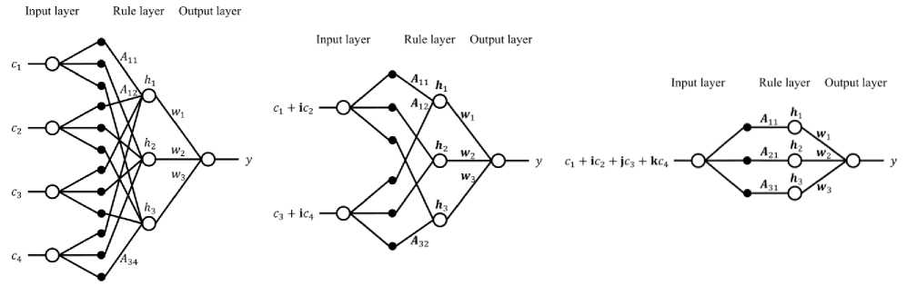
Fig. 3 illustrates SRNF, SCVNF, and SQNF for a problem heaving four real-valued inputs (c 1 , — ,c₄) and one output for better understanding of the proposed methods. The number of input nodes is four in SRNF, two in SCVNF, and one in SQNF. The number of divisions of each input space is three, then the number of rule nodes is three in SRNF, SCVNF, and SQNF.

In SRNF (Fig. 3(a)), the number of input nodes is four and each input space is divided into three. One membership function is used for each space to generate the antecedent grades. The weighted sum is applied to generate the output. The total number of membership functions is 3x4 = 12 (Л 11 , —, Л₃₄), and the number of antecedent grades is 3 (h 1 , —,h₃) which is equal to the number of rules. The number of parameters to be determined is 12x2 + 3 = 27.

In SCVNF (Fig. 3(b)), the number of input nodes is two and each input space is divided into three. One complex-valued membership function is used for each space to generate the complex-valued antecedent grades. The simplified gravity-like method as of Eq. (27) is used to generate the complex-valued net-input of output node. The activation function shown in Eq. (12) is used to convert the complex-valued net-input to real-valued output. The total number of complex-valued membership functions is 3x2 = 6 (Л11, •••, Л32), and the number of complex-valued antecedent grades is 3 (h1, —, h3) which is equal to the number of rules. The number of parameters to be determined is (6 x 2 + 3) x 2 = 30.

In the SQNF (Fig. 3(c)), the number of input node is only one and the input space is divided into three. One quaternion-valued membership function is used for each space to generate the quaternion-valued antecedent grades. The simplified gravity-like method as of Eq. (28) is used to generate the net-input of output node. The activation function shown in Eq. (21) converts the quaternion-valued net-input to real-valued output. The total number of quaternion-valued membership functions is 3x1 = 3 (Дц, — ,Д31) , and the number of quaternion-valued antecedent grades is 3 (h1, —, Л3) which is equal to the number of rules. The number of parameters to be determined is (3 x 2 + 3) x 4 = 36.

(b) SCVNF

(a) SRNF

(c) SQNF

Fig.3. Illustration of proposed SRNF, SCVNF and SQNF for a system with four real-valued inputs and one output. The number of divisions of each input space is three, then the number of rule nodes is three in each of them. The number of network parameters is 12×2+3=27 in SRNF, (6×2+3)×2=30 in SCVNF, and (3×2+3)×4=36 in SQNF.

• IV.    Experiments on Function Approximations

This section compares performance of each of proposed simplified methods SRNF, SCVNF, SQNF with its counter conventional method for function approximations. The following functions with two, four, and eight real variables are considered.

kx4,x5 + ix6 + jx7 + kx8). Table 2 shows the number of network parameters for each method. The number of divisions of each input space in the proposed methods is greater than that in the conventional methods. The numbers of divisions of each input for membership functions were determined by trial and error as shown in Table 2. The number of parameters is 2 x 52 x 2 + 52 = 125 in RNF, and 2x9x2 + 9 = 45 in SRNF.

fn1 :

у = (2sin(^x1) + cos(hx2))/6 + 0.5 ,

fn2 :

у =

(2. 1 +4.+^ ^ {(s^^^⁴)

74.42

4.68

—I

0.5

-0.077}

,

fn3 :

У = 2{

(2. 1 +4. 2 +0.1)²   {(3е^3х з +2е^— «⁴ ) 0.5 -,

0.077}

74.42

4.68

(2. 5 +4. 6 + 0.1)²  4 sin(^. y )+2 cos(^.₈)+6

37.21

;} •

Table 2. Number of Network Parameters for each of the Methods on Function Identifications

Dataset	Method	Input	Divisio n	Parameter *
fn1	RNF	2	5	2 x 5 2 x 2 + 5 2 = 125
	SRNF	2	9	2x9x2 + 9 = 45
fn2	CVNF	2	5	(2 x 5 2 x 2 + 5 2 ) x 2 = 250
	SCVN F	2	11	(2 x 11 x 2 + 11) x 2 = 110
fn3	QNF	2	5	(2 x 5 2 x 2 + 5 2 ) x 4 = 500
	SQNF	2	7	(2 x 7 x 2 + 7) x 4 = 140

*Parameter means total number of network parameters.

Here, Eq. (28) was used for SRNF and RNF, Eq. (29) for SCVNF and CVNF, and Eq. (30) for SQNF and QNF. As described in Section II, two real inputs were used as one complex-valued input in complex-valued methods, and four real inputs were used as one quaternion-valued input in quaternion-valued methods. Therefore, in the complex-valued SCVNF and CVNF methods, there are two complex-valued inputs (x 1 + ix₂,x₃ + ix₄), and in the quaternion-valued SQNF and QNF methods, there are two quaternion-valued inputs ( x 1 + ix₂ + jx₃ +

In this simulation, datasets with inputs and outputs made by each function were divided into training set (75%) and test set (25%). Two training datasets were made for each function as fn1.1, fn1.2, fn2.1, fn2.2, fn3.1, and fn3.2 with different samples. Computational time to train the network with training set was also computed as execution time. The experiments have been conducted on a single machine (HP Z440, Processor: Intel(R) Xeon(R) CPU E5-1603 v3 @ 2.80GHz, RAM: 32.0GB, SSD: 256GB); therefore, execution time comparison reflects computational efficiency of the methods. To measure the performance of method, the mean squared error (MSE) for test set was calculated as test error by

MSE=^Z^=i(dp-yp)2, (31)

where p is the pattern number, P is the total number of test patterns, d_p is the desired output, and y_p is the actual output.

Tables 3, 4, and 5 show the simulation results for comparison. The conventional and proposed methods were trained up to 10,000 epochs. The results showed that the proposed methods have the same convergence capabilities as the conventional methods. The proposed methods had fewer network parameters than the conventional methods (shown in Table 2), and the learning times were reduced (shown in Tables 3-5).

• V.    Experiments on Real-World Benchmark Problems

This section investigates the performance of the proposed simplified methods SRNF, SCVNF, SQNF on real-world benchmark problems. The description of the datasets and experimental setup is given first. The outcomes of proposed methods are then compared with conventional methods and another related prominent methods.

• A.    Description of the Datasets

Datasets from the UCI Machine Learning Repository [32] were used for the experiments. The repository is a collection of machine learning problems. Ten datasets for supervised learning were used. The short descriptions of these datasets are given below.

• 2)    Airfoil

This is a NASA dataset. The task is to calculate an airfoil self-noise level under different conditions for chord length, frequency, and other factors. There are 5 inputs, 1 continuous valued output, and 1,503 samples.

• 3)    Yacht

The task is to predict a residuary resistance of sailing yachts at the initial design stage. Essential inputs include the basic hull dimensions and the boat velocity. There are 6 inputs, 1 continuous valued output, and 308 samples.

• 4)    Concrete

The task is to calculate the compressive strength of concrete. This is a highly nonlinear function of age and ingredients, such as cement and water content. There are 8 inputs, 1 continuous valued output, and 1,030 samples.

• 5)    Turbine

The task is to compute a gas turbine’s compressor decay coefficient by numerical simulation of a naval vessel. The propulsion system behavior is described using components such as ship speed and turbine shaft torque. There are 16 inputs, 1 continuous valued output, and 11,934 samples.

• 6)    Iris

The task is to classify a type of plant. One class is linearly separable from the other two; the latter are nonlinearly separable from each other. It has 4 attributes, 3 classes, and 150 samples.

• 7)    Seed

The task is to classify three different varieties of wheat. Features consist of seven geometric parameters of wheat kernels. It has 7 attributes, 3 classes, and 210 samples.

• 8)    Diabetes

The task is to classify a patient as diabetes or not. Features include body mass index, diastolic blood pressure, triceps skin fold thickness, and so on. It has 8 attributes, 2 classes, and 768 samples.

• 9)    Cancer

This is a breast cancer dataset. The task is to classify a cell as benign or malignant. Features include clump thickness, cell size, bare nuclei, and so on. It has 10 attributes, 2 classes, and 683 samples.

Table 3. Average Test Error on fn1

Dataset	Test error ± S.D. (×10-3)		Execution time (s)
	RNF	SRNF	RNF	SRNF
fn1 .1	0.13 ± 0.02	0.36 ± 0.10	0.42	0.15
fn1.2	0.12 ± 0.02	0.34 ± 0.09	0.42	0.16

Averages and S.D.s were taken over 20 independent runs. S.D.: Standard deviation

Table 4. Average Test Error on fn2

Dataset	Test error ± S.D. (×10-3)		Execution time (s)
	CVNF	SCVNF	CVNF	SCVNF
fn2 .1	2.81 ± 0.21	2.72 ± 0.25	1.67	0.68
fn2.2	2.44 ± 0.19	2.44 ± 0.28	1.67	0.68

Averages and S.D.s were taken over 20 independent runs.

Table 5. Average Test Error on fn3

Dataset	Test error ± S.D. (×10-3)		Execution time (s)
	QNF	SQNF	QNF	SQNF
fn3 .1	1.69 ± 0.15	1.45 ± 0.17	4.44	0.95
fn3.2	1.69 ± 0.21	1.56 ± 0.17	4.44	0.94

Averages and S.D.s were taken over 20 independent runs.

• B.    Experimental Setup

In this experiment, each dataset was partitioned into training and test sets as in Table 6. Each of the datasets described above contain real-valued data. Attributes and class labels were respectively normalized in the ranges [– 1, 1] and [0, 1] for all datasets. For initialization, the number of network parameters for each of the methods was set as shown in Tables 7 and 8. Note that RNF could not be applied to the Turbine datasets, because of the huge number of parameters. Further, for the complex and quaternion-valued methods, the number of total parameters includes the real and imaginary parts of the parameters. As in the previous section, two real inputs were used as one complex-valued input in the complexvalued methods, and four real inputs were used as one quaternion-valued input in the quaternion methods. When the number of attributes of a dataset was not a multiple of two or four, empty parts of a complex or a quaternionvalued input variable were set to zero. For example, for Airfoil dataset with five attributes (c 1 , c₂, —,c₅) , the SCVNF and CVNF networks have three complex inputs

(x 1 = c 1 + ic₂,x₂ = c₃ + ic₄,x₃ = c₅ + i0) , and the SQNF and QNF networks have two quaternion-valued inputs (x 1 = c 1 + ic₂ + jc₃ + kc₄, x₂ = c₅ + i0 + j0 + k0).

Table 6. Partitioning of UCI Benchmark Datasets

Dataset Partitioning Name Attribute Class Total Training Testing Plant 4 Continuous 9568 7170 2398 Airfoil 5 Continuous 1503 1127 376 Yacht 6 Continuous 308 231 77 Concrete 8 Continuous 1030 772 258 Turbine 16 Continuous 11934 8950 2984 Iris 4 3 150 112 38 Seed 7 3 210 158 52 Diabetes 7 (8) a 2 768 576 192 Cancer 9 (10) a 2 683 512 171 Heart 13 2 270 202 68 a 7 of 8 attributes are used for Diabetes dataset, and 9 of 10 attributes are used for Cancer dataset.

Table 7. Number of Network Parameters for the Conventional Methods on Real-World Benchmark Problems

Dataset	RNF			CVNF			QNF
	Input	Division	Parameter	Input	Division	Parameter	Input	Division	Parameter
Plant	4	3	729	2	3	90	1	3	36
Airfoil	5	3	2673	3	4	896	2	3	180
Yacht	6	2	832	3	2	112	2	2	80
Concrete	8	2	4352	4	3	1458	2	3	180
Turbine	16	2	2162688	8	2	8704	4	3	2916
Iris	4	2	144	2	3	90	1	5	60
Seed	7	2	2176	4	2	352	2	3	252
Diabetes	7	3	32805	4	4	4608	2	9	1620
Cancer	9	2	9728	5	2	704	3	2	224
Heart	13	2	221184	7	2	3840	4	3	2916

Table 8. Number of Network Parameters for the Proposed Methods on Real-World Benchmark Problems

Dataset	SRNF			SCVNF			SQNF
	Input	Division	Parameter	Input	Division	Parameter	Input	Division	Parameter
Plant	4	11	99	2	3	30	1	2	24
Airfoil	5	41	451	3	11	154	2	11	220
Yacht	6	5	65	3	3	42	2	2	40
Concrete	8	11	187	4	11	198	2	4	80
Turbine	16	41	1353	8	41	1394	4	41	1476
Iris	4	2	18	2	2	20	1	2	24
Seed	7	11	187	4	11	242	2	4	112
Diabetes	7	11	165	4	11	198	2	2	40
Cancer	9	41	779	5	21	462	3	5	140
Heart	13	11	297	7	4	120	4	4	144

Each of the learning algorithms described in Section II (i.e., conventional methods) and Section III (i.e., proposed methods) was tested on the benchmark problems. During the training process, learning rates (a,f>,y) of the algorithms for each of the datasets were kept constant. Singletons were initialized with Gaussian random numbers. (ц,

(0,0.4).

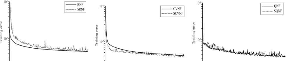
The proposed and conventional methods were trained using training sets for each of the problems up to 100000 epochs. When a network was trained with input and output patterns, the error on the training set decreased gradually with the epochs. During training, error for the training set was periodically computed by Eq. (4). The experiments have been conducted on the same machine described for function optimization.

Fig. 4 shows training processes for each of the methods on the Airfoil dataset. The proposed methods could converge as the conventional methods did. In the proposed methods, SCVNF and SQNF converged faster than SRNF. In this case, SQNF showed the minimum error among the proposed methods.

зобто ' 4<Лю ¹ ыйоо ' жЛ» ‘ louboo j зо^го ' 4* ¹ 6(А» ' soion ' loohon J ' зй» ' 4«ta ' sota ' sota ' iota ^                                           Epoch                                            Epoch

• (a) RNF and SRNF                (b) CVNF and SCVNF                (c) QNF and SQNF.

• Fig.4. Training process comparison on Airfoil dataset.

• C. Experimental Results and Comparison

This section compares the learning abilities of the conventional and proposed methods. To measure the performances, Eq. (31) was used to measure test error (MSE for test sets) for datasets with continuous output values. Accuracy rates were used for datasets for classification tasks. The accuracy is the ratio of the total number of classifications that are correct. The required training time for each method was also compared as execution time. Tables 9 and 10 summarizes the results for datasets with continuous output values, and classification tasks, respectively. These results were taken over 20 independent runs for each dataset.

In terms of the test error for continuous valued problem in Table 9, the proposed SRNF showed slightly better results than the conventional RNF did. In the best case, the test errors on Yacht dataset were 0.00397 for RNF, and 0.00141 for SRNF. Comparing the complex methods, the proposed SCVNF was slightly better than the conventional CVNF for most datasets. The proposed SQNF showed results similar to the conventional QNF.

Table 9. Average Test Error and Execution Time Comparison for Datasets with Continuous Output Values

Dataset

Test error ± S.D. (×10-3)

Execution time (s)

RNF

SRNF

CVNF

SCVNF

QNF

SQNF

RNF

SRNF

CVNF

SCVNF

QNF

SQNF

Plant

1.55 ± 0.01

1.63 ± 0.02

1.56 ± 0.02

1.65 ± 0.04

1.56 ± 0.02

1.64 ± 0.02

11.32

1.58

2.72

0.95

2.04

0.94

Airfoil

4.42 ± 0.08

3.99 ± 0.36

3.92 ± 0.31

4.14 ± 0.43

3.87 ± 0.47

3.49 ± 0.59

16.64

2.83

8.34

1.41

2.28

1.94

Yacht

3.97 ± 0.49

1.41 ± 0.69

1.90 ± 0.76

1.16 ± 0.29

0.79 ± 0.46

0.97 ± 0.23

1.92

0.17

0.50

0.19

0.55

0.20

Concrete

4.11 ± 0.23

4.07 ± 0.30

3.68 ± 0.68

3.47 ± 0.22

3.04 ± 0.28

3.59 ± 0.21

30.16

1.35

14.51

1.92

2.80

0.92

Turbine

*

0.62 ± 0.08

2.01 ± 1.07

1.38 ± 0.16

0.79 ± 0.31

1.02 ± 0.43

*

33.24

267.52

40.98

113.86

43.67

Averages and S.D.s were taken over 20 independent runs.

* The number of parameters was too large to perform calculation.

Table 10. Average Accuracy Rate and Execution Time Comparison for Classification Tasks

Dataset	Accuracy rate (%)						Execution time (s)
	RNF	SRNF	CVNF	SCVNF	QNF	SQNF	RNF	SRNF	CVNF	SCVNF	QNF	SQNF
Iris	100.00	100.00	100.00	100.00	100.00	100.00	0.15	0.05	0.22	0.06	0.28	0.08
Seed	92.40	90.96	91.83	89.90	91.44	90.77	9.24	1.20	3.85	1.20	2.69	0.80
Diabetes	75.89	72.81	74.19	74.48	75.76	74.58	200.20	0.54	42.14	0.88	5.73	0.25
Cancer	94.97	95.23	95.56	96.05	95.88	95.88	28.05	2.23	2.99	1.84	1.35	0.60
Heart	67.65	80.22	71.69	77.94	73.60	78.60	101.36	0.69	6.27	0.41	7.65	0.49

Averages and S.D.s were taken over 20 independent runs.

In terms of the accuracy rate of classification problem in Table 10, the proposed methods had almost the same performances as the conventional methods on Iris , Seed , Diabetes , and Cancer datasets. On Heart dataset, the proposed methods showed higher accuracies than the conventional methods.

In terms of the execution time in Tables 9 and 10, each of the proposed methods took less time than each of the conventional methods on all datasets. For example, on Plant dataset, the execution times were 11.32 sec for RNF, 1.58 sec for SRNF, 2.72 sec for CVNF, 0.95 sec for SCVNF, 2.04 sec for QNF, and 0.94 sec for SQNF.

Execution time relates to the computational complexity and the number of parameters in each method. As a simple example, a complex-valued multiplication needs around twice the computational time of a real-valued multiplication, whereas quaternion-valued multiplication needs around eight times. Proposed simplified methods had fewer computational complexities, and thus had less execution times in the experiments due to less parameters.

Table 11. Accuracy Rate Comparison of Proposed methods with NFRBC

Dataset	NFRBC	Proposed Method
Iris	80.87	100.00
Diabetes	75.03	74.58
Cancer	94.33	96.05
Heart	73.67	80.22

Finally, outcome of the proposed methods are compared with a recent neuro-fuzzy method [14] which applied a neuro-fuzzy rule-based classifier (NFRBC) to real-world classification problems with the UCI datasets. They used some of the datasets used in this study; Iris , Diabetes , Cancer , and Heart datasets. Thus, the proposed methods were compared with the NFRBC on these four datasets in Table 11. For the NFRBC, the best accuracy of Iris , Diabetes , Cancer , and Heart datasets were 80.87, 75.03, 94.33, and 73.67, respectively. On the other hand, for the proposed methods, the individual best accuracies for Iris , Diabetes , Cancer , and Heart datasets were 100.00, 74.58, 96.05, and 80.22, respectively. While this comparison was not necessarily strict, the proposed methods had higher accuracies than the NFRBC on three datasets except Diabetes dataset.

• VI. Conclusions

A simplified neuro-fuzzy method has been investigated in this study and incorporated in conventional methods. The conventional neuro-fuzzy methods, RNF, CVNF and QNF, suffer from the problem of increased number of parameters to be estimated by gradient descent method when the number of inputs is increased. Rules are made by all the combinations of membership functions in RNF; thus, the number of rules as well as total parameters increase rapidly with the number of inputs. In case of CVNF and QNF, although the total number of parameters is less than RNF due to their ability of solving a problem with less number of inputs, parameters increase with number of inputs. In the simplified method, the number of fuzzy rules is equal to the number of divisions of input space. And therefore, the number of rules as well as parameters are limited significantly in the proposed SRNF, SCVNF and SQNF in which the simplified method is incorporated in the conventional methods.

The proposed SRNF, SCVNF and SQNF are found to solve given problems with much less parameters as well as computing time with respect to their conventional counter methods. Total parameters of SRNF, SCVNF and SQNF were significantly less in number with respect to conventional RNF, CVNF and QNF, respectively for both function approximations (Table 2) and real-world benchmark problems (Tables 7-8). With much less execution times, proposed methods were competitive to conventional methods on test error and accuracy of the problems (Tables 3-5, Tables 9-10).

In the proposed SRNF, SCVNF and SQNF, the parameters such as the number of divisions can be chosen arbitrarily within a certain range. These properties provide a freedom in designing the system. In our numerical experiments, the network parameters for the RNF were difficult to determine, required trial-and-error, while those for SCVNF and SQNF were easy to fix. Further improvement is also possible in SCVNF and SQNF. The activation functions used to convert complex and quaternion values to real-valued output, Eq. (12) and Eq. (21), respectively, may be altered for better performance.

The proposed SRNF, SCVNF and SQNF have fewer parameters, and then systems with a larger number of inputs can be handled by the methods. Neuro-fuzzy can approximate certain types of nonlinear functions well in nature. Therefore, neuro-fuzzy models have been applied in designing control systems, such as the temperature control system for greenhouse [33], an antilock braking system of motor vehicle [34], a water-level control of U-tube steam generators in nuclear power plants [35], and so on [3, 7, 8]. This study have exhibited that proposed methods have better properties than the conventional counter methods in function approximations and real-world benchmark problems. Especially, they converge well in problems with a large number of inputs and the conventional methods are hard to apply. Therefore, the proposed methods can be utilized for the large problems (e.g., real-time control of large systems) where the conventional methods are difficult to apply due to time constrain.

This work was supported by the Grants-in-Aid from JSPS; Nos.15K00333 for KM and 16J11219 for RH. The funding source had no role in study design; in the collection, analysis and interpretation of data; in the writing of the report; and in the decision to submit the article for publication.

• [1]    J. S. Jang and C. T. Sun, “Neuro-fuzzy modeling and control,” Proceedings of IEEE , vol. 83, no. 3, Mar. 1995.

• [2]    G. Feng, “A survey on analysis and design of modelbased fuzzy control systems,” IEEE Transactions on Fuzzy systems , vol. 14, no. 5, pp. 676–697, Oct. 2006.

• [3]    S. Kar, S. Das, and P. K. Ghosh, “Applications of neuro fuzzy systems: A brief review and future outline,” Applied Soft Computing , vol. 15, pp. 243–259, Feb. 2014.

• [4]    M. Ababou, M. Bellafkih and R. E. Kouch, “Energy Efficient Routing Protocol for Delay Tolerant Network Based on Fuzzy Logic and Ant Colony,” I. J. Intelligent Systems and Applications , vol. 10, no. 1, pp. 69-77, 2018.

• [5]    A. Amini and N. Nikraz, “Proposing Two Defuzzification Methods based on Output Fuzzy Set Weights,” I. J.

Intelligent Systems and Applications , vol. 8, no. 2, pp. 112, 2016.

• [6]    N. Arora and J. R. Saini, “Estimation and Approximation Using Neuro-Fuzzy Systems,” I. J. Intelligent Systems and Applications , vol. 8, no. 6, pp. 9-18, 2016.

• [7]    Z. Hu, Y. V. Bodyanskiy, N. Y. Kulishova and O. K. Tyshchenko, “A Multidimensional Extended Neo-Fuzzy Neuron for Facial Expression Recognition,” I. J. Intelligent Systems and Applications , vol. 9, no. 9, pp. 2936, 2017.

• [8]    N. H. Saeed and M. F. Abbod, “Modelling Oil Pipelines Grid: Neuro-fuzzy Supervision System,” I. J. Intelligent Systems and Applications , vol. 9, no.10, pp. 1-11, 2017.

• [9]    Y. Shi, M. Mizumoto, N. Yubazaki, and M. Otani, “A method of fuzzy rules generation based on neuro-fuzzy learning algorithm,” Fuzzy Theory Systems , vol. 8, no. 4, pp. 103–113, Aug. 1996.

• [10]    Y. Shi, M. Mizumoto, N. Yubazaki, and M. Otani, “A learning algorithm for tuning fuzzy rules based on the gradient descent method,” Proceedings of the Fifth IEEE International Conference on Fuzzy Systems , 1996, pp. 55– 61.

• [11]    Y. Shi and M. Mizumoto, “A new approach of neuro-fuzzy learning algorithm for tuning fuzzy rules,” Fuzzy sets and systems , vol. 112, no. 1, pp. 99–116, May 2000.

• [12]    W. Wu, L. Li, J. Yang, and Y. Liu, “A modified gradientbased neuro-fuzzy learning algorithm and its convergence,” Information Sciences , vol. 18, no. 9, pp. 1630–1642, May 2010.

• [13]    K. Shimojima, T. Fukuda, and Y. Hasegawa, “RBF-fuzzy system with GA based unsupervised/supervised learning method,” Proceedings of 1995 IEEE International Conference on Fuzzy Systems , 1995, vol. 1, pp. 253–258.

• [14]    J. Kim and N. Kasabov, “HyFIS: adaptive neuro-fuzzy inference systems and their application to nonlinear dynamical systems,” Neural Networks , vol. 12, no. 9, pp. 1301–1319, Nov. 1999.

• [15]    A. Bhardwaj and K. K. Siddhu, “An Approach to Medical Image Classification Using Neuro Fuzzy Logic and ANFIS Classifier,” International Journal of Computer Trends and Technology , vol. 4, no. 3, pp. 236–240, 2013.

• [16]    S. Ghosh, S. Biswas, D. Sarkar, and P. P. Sarkar, “A novel neuro-fuzzy classification technique for data mining,” Egyptian Informatics Journal , vol. 15, no. 3, pp. 129–147, Sept. 2014.

• [17]    P. Naresh and R. Shettar, “Image processing and classification techniques for early detection of lung cancer for preventive health care: A survey,” International Journal on Recent Trends in Engineering & Technology , vol. 11, no. 1, pp. 595–601, July 2014.

• [18]    S. Ghosh, S. Biswas, D. C. Sarkar, and P. P. Sarkar, “Breast cancer detection using a neuro-fuzzy based classification method,” Indian Journal of Science and Technology , vol. 9, no. 14, Apr. 2016.

• [19]    S. K. Biswas, M. Bordoloi, H. R. Singh, and B. Purkayastha, “A neuro-fuzzy rule-based classifier using important features and top linguistic features,” International Journal of Intelligent Information Technologies (IJIIT) , vol. 12, no. 3, pp. 38–50, Sept. 2016.

• [20]    J. E. Nalavade and T. S. Murugan, “HRNeuro-fuzzy: Adapting neuro-fuzzy classifier for recurring concept drift of evolving data streams u sing rough set theory and

  holoentropy,” Journal of King Saud University-Computer and Information Sciences , Nov. 2016.

• [21]    H. R. Singh, S. K. Biswas, and B. Purkayastha, “A neuro-fuzzy classification technique using dynamic clustering and GSS rule generation,” Journal of Computational and Applied Mathematics , vol. 309, pp. 683–694, Jan. 2017.

• [22]    K. Subramanian, R. Savitha, and S. Suresh, “A complexvalued neuro-fuzzy inference system and its learning mechanism,” Neurocomputing , vol. 123, no. 10, pp. 110– 120, Jan. 2014.

• [23]    C. Li, T. Wu, and F. T. Chan, “Self-learning complex neuro-fuzzy system with complex fuzzy sets and its application  to adaptive image noise canceling,”

Neurocomputing , vol. 94, no. 1, pp. 121–139, Oct. 2012.

• [24]    R. Hata, M. M. Islam, and K. Murase, “Generation of fuzzy rules based on complex-valued neuro-fuzzy learning algorithm,” 3^rd International Workshop on Advanced Computational Intelligence and Intelligent Informatics (IWACIII 2013) , 2013, GS1-3_D13070130.

• [25]    R. Hata and K. Murase, “Generation of fuzzy rules by a complex-valued neuro-fuzzy learning algorithm,” Fuzzy Theory and Intelligent Informatics , vo. 27, no. 1, pp. 533– 548, Mar. 2015.

• [26]    R. Hata, M. M. Islam, and K. Murase, “Quaternion neuro-fuzzy learning algorithm for fuzzy rule generation,” Proceedings of the Second International Conference on Robot, Vision and Signal Processing (RVSP 2013) , 2013, pp. 61–65, Dec. 2013.

• [27]    R. Hata and K. Murase, “Quaternion neuro-fuzzy for realvalued classification problems,” Proceedings of the Joint 7th International Conference on Soft Computing and Intelligent Systems and 15^th International Symposium on Advanced Intelligent Systems (SCIS&ISIS 2014) , 2014, pp. 655–660.

• [28]    R. Hata, M. M. Islam, and K. Murase, “Quaternion neuro-fuzzy learning algorithm for generation of fuzzy rules,” Neurocomputing , vol. 216, pp. 638–648, Dec. 2016.

• [29]    R. Hecht-Nielsen, “Theory of the backpropagation neural network,” Proceedings of International Joint Conference on Neural Networks , 1989, pp. 593–605.

• [30]    M. F. Amin and K. Murase, “Single-layered complexvalued neural network for real-valued classification problems,” Neurocomputing , vol. 72, no. 4, pp. 945–955, Jan. 2009.

• [31]    M. F. Amin, M. M. Islam, and K. Murase, “Ensemble of single-layered complex-valued neural networks for classification tasks,” Neurocomputing , vol. 72, no. 10, pp. 2227–2234, June 2009.

• [32]    K. Bache and M. Lichman, UCI Machine Learning Repository , Univ. California, Irvine, CA, USA, 2013.

• [33]    D. M. Atia and H. T. El-madany, “Analysis and design of greenhouse temperature control using adaptive neuro-fuzzy inference system,” Journal of Electrical Systems and Information Technology , Oct. 2016.

• [34]    C. M. Lin and C. F. Hsu, “Self-learning fuzzy slidingmode control for antilock braking systems,” IEEE Transactions on Control Systems Technology , vol. 11, no. 2, pp. 273–278, Mar. 2003.

• [35]    S. R. Munasinghe, M. S. Kim, and J. J. Lee, “Adaptive neurofuzzy controller to regulate UTSG water level in nuclear power plants,” IEEE Transactions on Nuclear Science , vol. 52, no. 1, pp. 421–429, Feb. 2005.

Authors’ Profiles

Ryusuke Hata received his M.E. and Ph.D. in Human and Artificial Intelligent Systems in 2014, and the Ph.D. in System Design Engineering in 2017 from University of Fukui, Japan. His research interests include neural networks, fuzzy logic, and autonomous systems.

M. A. H. Akhand received his B.Sc. degree in Electrical and Electronic Engineering from Khulna University of Engineering and Technology (KUET), Bangladesh in 1999, the M.E. degree in Human and Artificial Intelligent Systems in 2006, and the Ph.D. in System Design Engineering in 2009 from University of Fukui, Japan.

He joined as a lecturer at the Department of Computer Science and Engineering at KUET in 2001, and is now a Professor and Head. He is also head of Computational Intelligence Research Group of this department. He is a member of Institution of Engineers, Bangladesh (IEB). His research interest includes artificial neural networks, evolutionary computation, bioinformatics, swarm intelligence and other bioinspired computing techniques. He has more than 50 refereed publications.

Md. Monirul Islam received his B.E. degree from the Khulna University of Engineering and Technology (KUET), Khulna, Bangladesh, in 1989, his M.E. degree from the Bangladesh University of Engineering and Technology (BUET), Dhaka, Bangladesh, in 1996, and his Ph.D. degree from the University of Fukui, Fukui,

Japan, in 2002.

From 1989 to 2002, he was a lecturer and an assistant Professor with the KUET. Since 2003, he has been with the BUET, where he is currently a professor with the Department of Computer Science and Engineering. He was a visiting associate professor with the University of Fukui. His current research interests include evolutionary robotics, evolutionary computation, neural networks, machine learning, pattern recognition, and data mining. He has over 100 refereed publications in international journals and conferences.

Kazuyuki Murase received his M.E. degree in electrical engineering from Nagoya University, Nagoya, Japan, in 1978, and his Ph.D. degree in biomedical engineering from Iowa State University, Ames, IA, USA, in 1983.

He was a Research Associate with the Department of Information Science, Toyohashi University of Technology,

Toyohashi, Japan, in 1984, and an Associate Professor with the

Department of Information Science, Fukui University, Fukui, Japan, in 1988, and became a Professor in 1993. He served as Chairman of the Department of Human and Artificial Intelligence Systems, University of Fukui in 1999. His current research interests include neuroscience of sensory systems, selforganizing neural networks, and bio-robotics.