Simulation Based Comparison of Geo-Location Methods in Wireless Networks

Published Online January 2015 in MECS

Day by day developing of wireless communication systems and cellular networks along with increasing demands for location based services make policy makers and implementers of wireless networks to improve and develop positioning techniques and algorithms in such networks. In addition FFC 1 regulations such as E-911 2 and emergency aids help to make this process faster and faster[1]. These aids can help users efficiently by ALI3. Therefore communication companies are looking for corresponding methods and algorithms that both more accurate and cheaper and easier to implement on hardware.

Mainly there are two methods for user Geo-location. The first help the use of GPS devices called GPS aided. Each has its own advantages and disadvantages, for example for indoor Geo-location GPS cannot be useful. Replacing the role of satellites in the GPS service by that of base stations, the second method appears. This method uses the signals exist inherently in underlying communication network and tries to estimate user position by observing parameters that are dependent to location. This method can furthermore divides in two main approaches; mobile based and network based. The difference is the roles of mobile station and BTS in measuring the signals and estimating/calculating the location. In this paper we focus on mobile based techniques.

To determine the user location, two main steps should be passed, the first is measuring some signals and estimating the location dependent parameter or parameters from them. The second step is to use an algorithm to calculate (better to say again estimating ) the position. Many texts including thesis and book chapters discussed different methods of first steps [2,3,4,5,6,7,8]. These methods exploit measuring of parameters such as TOA4, TDOA5, AOA6, RSS7, DCM8, TA9 and other hybrid models. The second step may help the use of many algorithm such as Filtering methods , estimation based method and meta heuristic and evolutionary algorithms and some other approaches which are discussed here. Because of different simulation methods and sceneries it is not possible to compare these algorithms just by looking at the results of papers. They should be compared under unique simulation environment so we decided to have a performance evaluation between them. In this paper, Geo-location methods are classified based on mathematical algorithms used to find user location in the both area of deterministic and stochastic approaches, these algorithms can then use with the same parameter so comparison between them is rational and possible. Such algorithms divided into 3 main subclasses, estimation theory based (MUSIC, ESPIRIT), Meta-heuristic (Genetic, PSO, ...) and filtering approaches (Kalman, Particle, Grid, MH ).

The contribution of this paper is to 1). Classifying Geo-location techniques based on mathematical approaches 2). Applying Simulation to them in the same environment 3). Comparing them based on both Radial Error and computational Complexity for implementation issues on hardware.

The rest of this paper is organized as follow: section 2 describes the methods based on Estimation theory, in section 3 , Meta-heuristic algorithms are presented and section 4 gives the information and different classes of Bayesian filtering in positioning. Finally in section 5 simulation details are described and some conclusions are given in section 6.

II. E stimation T heory B ased L ocalization M ethods

Many algorithms in the class of estimation theory have been developed for location estimation. The most fundamental algorithms is based on Maximum Likelihood and Maximum A posterior Probability techniques and the their derivatives. MUSIC 10 and ESPIRIT 11 are two of more popular. They use for so called "super resolution " estimation. Many variants of the two including fast versions, MIMO versions , adaptive and smart ones are applied to location estimation for estimating TOA,DOA12 and other parameters [5, 9, 10, 11,  12,  13,  14]. Both of them are essentially for estimating the frequencies of the signals. For example the first one, MUSIC, is based on linear algebra and vector space. If it is supposed that a signal is consist of desired signal and additive noise and composed of L single tones:

L u (n) = ^piej60^2 (n)                           (1)

i — ?

Then the covariance matrix of signal samples, R, can be decomposed in the following way [6]:

Where X_t and ^_t are respectively the Eigen values of matrix R and SD S^H ordering in the ascending manner. Because all of Eigen vectors of a matrix form a perpendicular space, the two subspace must be orthogonal to each other. So the MUSIC algorithm is looking for a frequencies that are in the signal plus noise subspace and are orthogonal to the noise subspace. So the frequency sweep matrix, S(u)), are defined to ensure which frequencies have the mentioned property. Thus the MUSIC Spectrum can easily be defined as:

SMUSIC (o)   HI           I \ s (°) VwVN s (°)

Where is the noise subspace vector. Each VN frequency having the peak value in the spectrum is in the signal frequency matrix. Some other versions such as Root-MUSIC and so on are also derived. By reciprocating the role of time and frequency one can easily apply these algorithm for TOA or in the same manner for DOA and so forth.

R = SDS H + ст ² 1

Where S is the frequency matrix, D is the diagonal Correlation matrix of single tones and a2 is the noise variance. They can be written in the following way:

III. M eta -H euristic L ocalization M ethods

There are also many papers focusing on meta-heuristic and evolutionary algorithms to solve the final positioning equation. Their main idea is the same, defining the objective or fitness function and solving the optimization (min/max) problem by the corresponding algorithm operators [15, 16, 17, 18,19,20].

Mainly the objective function is defined based on the mean square error of population fitness and observed one as :

F = min

Cell _ No

^ SSSE к i = 2

S = [ s i , s 2 ,..., s l ]   =

e " °'    e - ° e - j2o0    e - j 2°2

e " joL e "j °

For example in the case of TDOA, the difference distance of user location from reference BTS and the other is calculated as observed fitness and compared to that of for population generated by the algorithm.

e — jM o i   e — j^M ® i

e - ^jM ° L

D — diag ( P i ,P 2 , _ , P l )                        (3)

It can be shown that Eigen values of matrix R can be divided in to two subspace, signal plus noise and noise as described below:

_ _      (A

S S E — x • i x n /• 1

к cr , 1 ,1    Real_Cord , i ,1 J

(A

+ l ycr,i,1 yReal^     ,,i,1 I к ,,           Cord,, J

^ i =\

№ + ^ст i ; ст ² i ;

i = 1,2,-, L i = L +1,---, M

• ¹⁰    Multiple signal Classifier

• ¹¹    Estimation of Signal Parameters via Rotational Invariance Technique

• ¹²    Direction of arrival

Where x _{cr , i ,1} is a difference distance between current population and reference ( indexed here by 1) and ith base station on x-axis and x          is a real difference

Rea l_Cord , i ,1

distance (computed from measured TDOA values) of user and those base stations on x axis (so as ycr,i,1 and yReal   ,i,1 on y-axis). So the algorithm starts to find the best point that is as close as possible and enough to the collision point of mentioned hyperbolic curves.(note that

in the case of TDOA, the final positioning equation leads to intersection of two or more hyperbolic function. The operators in GA13 for example is selection, mutation and cross over to generate new generation. In the PSO14 there are velocities and position to be updated and help converge the solutions. What is really obvious is that none of these algorithms is suitable for online positioning systems, so they are not considered so much.

• IV.    B ayesian F iltering M ethods

There are different problems can be considered in the field of estimation [21], namely:

The prediction problem , concerned with the determination of

^{П (} Xk । Z I*k - I )

The filtering  problem,   concerned with the determination of

• * ( X k | Z_{L k} )

The fixed-lag smoothing problem , concerned with the determination of

” ( Xk|Z 1: k+p )  P>0

where X_k is the State vector in the time instant k and Z _{1? ? k} is all the measurement from time instant 1 to k. It is supposed to exist two equations or models: state update (evolution) model (equation) :

Xk = fk (Xk-1) + process_noise and measurement model (equation) :

Z _k = h_k ( X _k ) + Measurement _ noise

By using the Bayes formula the process of filtering can be decomposed into two steps: 1- State prediction sometimes called prediction 2- measurement update sometimes called correction. These steps are well illustrated in the Fig.1.

Bayesian filtering is a technique that is used for dynamic state estimating of a system with the help of some parameters observed in the presence of noise called noisy measurements. When a system is time variant many estimation algorithms cannot work well [22, 23].

If we define the Belief as below:

Bel ( X_k ) = n ( X k Z_k )

then the two mention steps are mathematically derived in this manner :

• 1-    prediction step:

Bel - = j ⁿ ( X k I x k - 1 ) ^Bel ( x k - 1 ) dx k - 1

• 2-    measurement update :

Bel ( x ,) = C, ?(Z_fc ? x_k)?Bel ? - ( x ,) tv tv tv tv                       tv

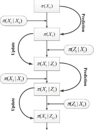
Fig. 1 prediction and update steps in Bayesian filtering

The prediction step is derived by applying the conditional and marginal probability theory :

Be1 " (Xk ) = *(X^Z»-1)

J ⁿ ( Xk I x k - I , ^Z 1 k - I ) ⁿ ( x k - I | ^Z l: k - I ) dx k - I

Where the first and second term in the integral are equal to n ( X _k | x _k - 1 ) and Bel ( x k - 1 ) respectively because x k - 1 and Z 1: _k - 1 has the same information due to the measurement equation) measurement update step is also derived by the Bayes rule. Note that the first step practically calculates (estimates) the state variables regarding behavioral action of state variables that state equation shows (regardless of incoming measurement and the second step updates and corrects the last values by the current measurement observed.

In this concept and in the case of localization and also other applications such as tracking [24,25,26], 3 popular methods are well discussed in the literature, Kalman filter ( and its derivatives EKF 15 ,UKF 16), Particle filter and Grid based method. Usually the EKF, UKF, Particle filter and Grid algorithm are classified in the approximation methods. Another classification is divided these methods in two categories continuous and discrete. Based on this, Kalman, EKF and UKF are continuous and Particle filter and Grid algorithm are discrete.

• ¹⁵    Extended kalman filter

• ¹⁶    unscented kalman filter

• A.    Kalman Filtering

If the state and measurement equations are linear correspond to state variables (f and h are linear functions)and the noise (process and measurement) is assumed to have normal distribution, Bayesian filtering converts to Kalman filtering [7, 27] with the solution derived by Kalman. In this case the two equations can be written in a matrix form. If the equations are not linear, then to have the previous solutions for the problem, first and second order of Taylor series approximations are used instead. In this case the corresponding Jacobean matrix is replaced. That is why these methods are called approximated.

For Kalman filtering to become an efficient estimator for localization problems, the dynamic state equation must be modeled accurately. There are many models developed in this case. Some of them are deterministic and the others are stochastic. Deterministic models exploit the Newton motion models ( position, velocity and acceleration equations) and simple and efficient to use.[ 27, 28]. For example Newton equations states that:

1       7

X = X + V A t + -a A t2

V = V0 + a A t

a (t) = a wiener process. These are more complex than the previous models [27, 28].

Measurement equation in the Kalman filtering depends on the observed parameters in the cellular network which can be TOA, RSS, TDOA, and so on discussed before. This equation could be either linear (in the case of TOA as an example) or nonlinear ( in the case of RSS for example) so for the former case the problem is the exact Kalman filtering and for the latter case EKF could be used to solve. As an example of EKF, in the case of RSS, measurement models exploit different propagation path loss models along with shadowing effect[ 29, 30, 31, 32]. One simple model could be written in the form :

Z k , i = Z o, i - 10 a log !o ( d k , i ) + v k , i (8)

Where is the path loss exponent (PLE), , is the received power from ith BTS at time k, , is the distance between mobile station and ith BTS and , is the noise value in ith link that is called shadowing and has lognormal distribution. it is completely nonlinear and must be approximated by Taylor series to be used by kalman technique called EKF. In this case The matrix form, the coefficient matrix of measurement equation achieved based on Jacobean definition discussed earlier :

H = In ( 10 ) * G

Hence the state variables could be position and velocity and acceleration in both x and y directions (in

2D scenario). Thus the matrix form of state equation is:

where G is :

X

= AX_k - 1 + noise

,,

=      ,,

,,

0  log(1)

0  log(2)

0  log(3)

)

Where

X k =

pk

Ук vxk vyk axk v ayk , and

A =

< 1 0 A t 0 | A t2 0 0 1 0 A t 0 1A t 0 0 1 0 At 0 0 0 0 1 0 At 0 0 0 0 1 0 V 0 0 0 0 0 1 is the state vector and A is the coefficient matrix of state equation Note that if each of velocity and acceleration terms does not come in the state vector as state variable, their impact should be modeled in the process noise.

Stochastic methods are usually use the Stochastic processes such as Random walk, Brownian motion and gi,1 = (x-xbi)/(di2 )

g i ,2 = ( У ^- ybi ) / ( ^{di 2} )

As it is seen in this case the path loss exponent is also brought in the state vector as state variable so that it can be estimated. and in the above equation is user coordination and (    ,    ) is the ith BTS coordination.

• B.    Grid method and Particle filtering

In these methods their algorithm tries to estimate posterior probability density function (PDF) in the state space and finds its maximum ( or calculates weighted average of the state space points ) as the final solution, it is a kind of MAP technique that best estimates the solution. The starting point of these algorithms is based on the below equation:

P (z | x) P (x)

P ( x | z ) = ^V      \     ^ ^P ( z ¹ x ) P ( x )           (10)

P(z)

where x and z are respectively state vector and measured parameter. () is called prior information. So firstly the solution space (state space) should be approximated in some points, that is why these methods are classified as discrete [32, 33]. Based on how the initial points for state space created, Grid or Particle method is emerged. If the space is uniformly divided it is called Grid, as its name implies, so there is a Grid like space to search for the optimal solution. Otherwise if the points in the solution space are created based on the prior probability distributed function particle filter is emerged.

For example in Grid method if the solution space is 1D, then the mentioned PDF would be something like Fig.2, then mathematically it is possible to state the posterior probability in terms of sum of weighted and shifted delta functions.

Fig. 2 uniformly partitioned 1D state space based on Grid

The main idea of particle filtering generating a set of likely points for solutions in the state space and representing the probability distribution function only in those points by assigning and calculating a weight to each point and normalizing the weights. The set of points are generated by the prior information, it means, the more points are generated in the region with more probability for user to be there. In other words, some point in the solution space are generated according to prior PDF and then for each point, a corresponding weight is calculated and again the prior PDF is updated according to the resulting weights, repeating this process yields the solution. Calculating the weights is based on measurements. Mathematically suppose {x Q. _k, w Q } ; i = 1 ,..., N_s , to be the set of points and corresponding weights in the state space. The index i is for points and index k is for time. The weights are normalized so that E j w Q = 1 . The posterior probability is defined as follows [33, 34]:

N

P ( x 0: k ^|z1: k ^^ wk ⁵ ( ^x 0: k - ^x 0: k )       ⁽¹¹⁾

Which is approximated version of the real and continuous posterior probability. In the case that the weights cannot be calculated easily or generating the set of points according to the prior information is not possible, the importance sampling technique is used. For a particle filter to be efficient, the points which is generated in the state space should have as high weights value as possible to prevent degeneracy problem. One way of preventing the generation of low valued weights is resampling. Resampling means directly omitting the points with low valued weights and replacing them by high value weights point. Fig. 4 illustrates this process[35] .

An example of particle filtering process in positioning with RSS parameter is developed in the simulation section with more details.

• C.    Metropolis Hastings Algorithm

This algorithm is basically used for generating random numbers with a target distribution and is in the class of Markov chain Monte Carlo method that uses acceptance rejection techniques to produce random numbers. It starts with generating a random number say x' from proposal distribution Q(x|y) and suppose target distribution is я(x) and the initial state is known and equal to x=x₀. If we define the ratio :

r ( x , x ') =

n (x') q (x|x') n (x) q (x '| x)

Then x= x' is the next state with the probability of r(x, x ' ) otherwise the previous state (here x₀) is chosen for the next state. This algorithm converge to the final solution[35, 36].

But what is the application of this algorithm in positioning? See simulation section for details.

• V.    S imulations A nd R esults

In this section some of popular methods have been simulated under the same and certain conditions to have a proper comparison. RSS measurement is used as observation parameter.

• A.    Network Model

To simulate the cellular network 3G system UMTS is chosen. A main cell and its 6 neighboring cells in the form of hexagonal shape is considered in MATLAB. See Fig.4.

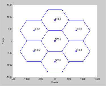
Fig. 4 Network model

UMTS Physical layer considering common pilot channel, Spreading codes and root raised cosine filtering is programmed. Cost 231 Hata model is used for path loss and shadowing with log-normal distribution with zero mean and 4 - 6 dB as variance added. Multipath fading is also simulated with 3 paths and Doppler frequency of 50Hz. Furthermore TA-IPDL is used for hearability problem. Because of symmetric form of network, the position for user is generated randomly in a triangle shown in the Fig.5. So to generate a position for user location uniformly in the shown triangle, the X and Y coordinates must be generated using below distribution:

X = R * ( U ) whereU-Uniform ( 0.1 )     (13)

Y = 3XX + V where

V~Uniform ( 0,43 * ( R - X ) )             (14)

And R is the cell radius.

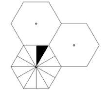
Fig. 5 symmetric form of cell and generating uniformly user position

Proof : The objective is to generate position uniformly in the black triangle therefore the joint distribution of X,Y is:

^f x , y

84г 0 <  X < R and 3XX <  Y <  3 R R

3 R ^{2   22}

0 otherwise

One easy way is to produce X coordinate uniformly in the interval 0 < < . then according to the conditions on Y, Y can be written in the form = √3 + but V can gets values such that the values of Y lies in its min/max constraints, i.e., V can have values between 0 and ^√ R - √3 X .

• B.    Kalman filtering simulation

According to (8) and (9), both position and path loss exponent are estimated in this simulation. At first a fixed user is simulated and in another simulation a path with discontinuity is assigned to the user and the corresponding RSS with path loss model (cost 231 Hata) are fed to the Kalman routine to estimate the position. Fig.6, Fig.7 and Fig.8 show the process.

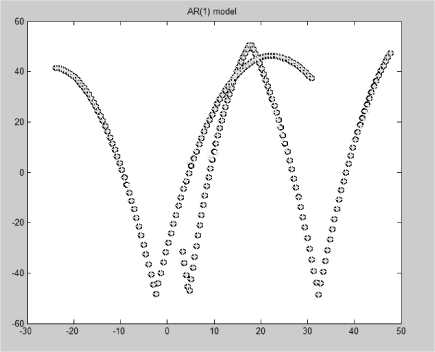
Fig. 6 path with discontinuity is assigned to the user motion

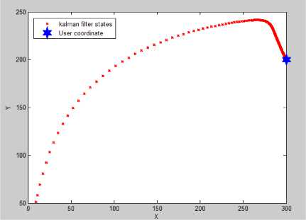
Fig. 7 Fixed user location Estimation

• C.    Genetic algorithm Simulation

  The objective function of genetic algorithm is set according to (6) and (7). The other parameters are : Population size = 1000, Generation size= 1000; fitness

limit = 1 e -5, Tolerance function between successive generations = 1 e -10 . Fig.10 shows the process.

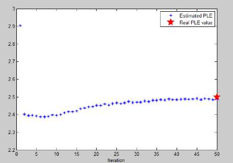
Fig. 8 Path loss exponent estimation

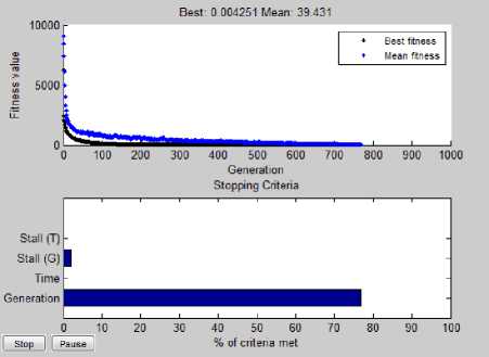
Fig. 9 Genetic algorithm fitness and generations plot

As stated before evolutionary algorithms is not suitable for real time processing because they are usually timeconsuming. Here , the process of converging to the solution is so long if precise solutions are considered.

• D.    Particle filter simulation

For the simulation of particle filtering, 2 normal distribution with means equal to the main BTS coordination and standard deviation order of cell radius (R or R/2) is firstly chosen. Then 200 points for X and Y are generated and each is assigned a weight according to P( _∶ │ ), where is the position of i^th point and n is the number of BTS that they are observed by the mobile station.. note that this is likelihood function not posterior, but because the choosing point algorithm is used then the total process yields posterior distribution. Because the measurements of different BTS are independent then:

n

^P ( z 1: n lx ) = H P ( z j |P i ) ⁽¹⁶⁾ j = 1

and according to the (8) , P(z|p) has log-normal distribution with mean 10 α ln(d) and variance equal to that of shadowing. After calculating the weights for each points, the weighted average is used for estimating the position for first iteration. For the second iteration, 200 points are drawn from the normal distribution with mean equal to the estimating position achieved from the first iteration. And the process goes for merely 2 or 3 iterations to reach the best point. Fig.10, Fig.11 and Fig.12 show the process, in this simulation the user location is in x= 100,y= 200 and R= 500. As it is shown the posterior PDF is going through the real position . For the second and third iteration, the same data size (200 points) are produced via random number generating algorithms extracting the normal random numbers but with the updated variance and mean from the data and their weights of the last iteration. (Mean and variance should be calculated regarding the weights of each point ).

• E.    Metropolis Hastings simulation

In the positioning target distribution is the posterior probability:

п ( X )= P (( p^vn ))                              (17)

where p is the user position and y _∶ is received power of n BTS's. Proposal distribution q(р′|p ) is defined as normal with mean p and standard deviation which is order of cell radius (R or R/2):

q ( p 1 p ) = N ( p k - 1 , a² )

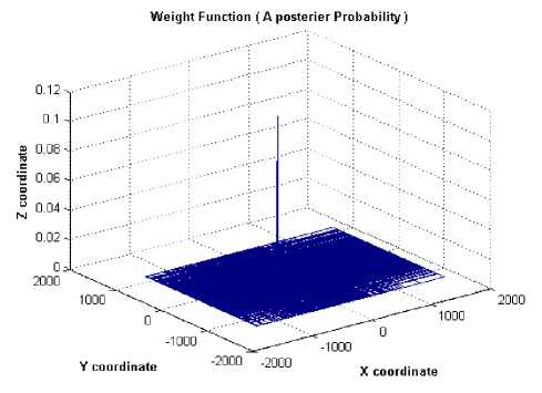
Fig. 10 posterior approximation after iteration 1

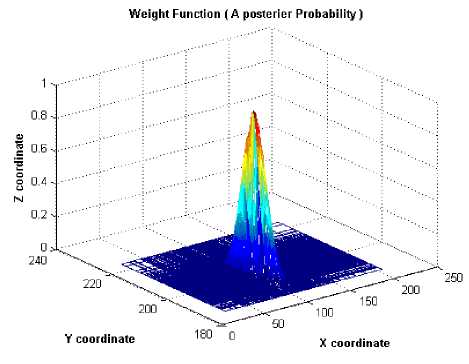
Fig. 11 posterior approximation after iteration 2

Weight Function (Д posterior Probability)

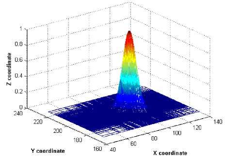
Fig. 12 posterior approximation after iteration 3

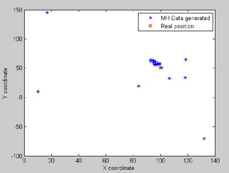
Fig. 13 MH generating points for location estimation

So by this assumptions the corresponding ratio of MH17 algorithm is :

r ( P k - 1 ,p ' )

^P ( ( p ' I У 1: » ) ) q ( P k - 1 1 p' )

^P ( ( P k - 1 | У 1: n ) ) q ( P'|P k - 1 )

where p' is the next generated point from proposal distribution, p is the last accepted point and p is the initial point. The outstanding property of normal distribution is manifested here. q(p |p′) and q(p′|p ) has the mean p' and p respectively and they have the same values in the point p and p' . so we have

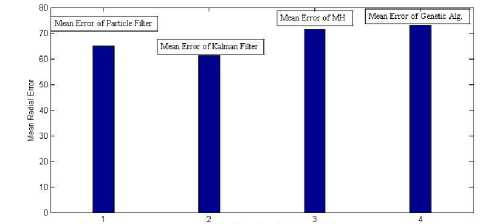
The radial Error of each algorithm is thus plotted in the Fig.14. Note that these errors are obtained from running the simulation for 1000 times. As it is shown in theFig.15, the best method in the case of radial error is EKF, but it is obvious that the performance of each method is highly dependent on the time and resources it needs. But we can say the EKF is again the best method in the case of computational complexity either. Even MH algorithm which seems to be less complex requires many iterations (more than 500,000 in the case of 4 state variables) to converge to the solution as the number of state variables goes high.

^r ( p k - 1 ,p ' ) =

^P (⁽ Р'|У 1: n ) )

^P ( ( P k - 1 |У 1: n ) )

To calculate the numerator of the above ratio, Bayes rule is applied:

P (( p‘|y1: n )) =

P ( У1: nip’) P ( P ‘) P ( У1: n )

* P ( У1: n| p‘) P ( P')

And for the denominator:

P (( pk-1У1:п )) =

^P ( У 1: n |p k - 1 ) ^P ( p k - 1 ) ^P ( У 1: n )

^ ^P ( У 1: n |p k - 1 ) ^P ( p k - 1 )

From (8) and independent assumption of incoming

signal from different BTS,:

n

^P ( У 1: n |p' ) = n P ( У j ^|P' )

j = 1

And P(y |p′) is log-normal with mean 10 α ln(d′) and variance equal to that of shadowing. Fig.13 shows the MH process.

17 Metropolis Hastings

inde« of method

Fig. 14 Radial Error of different positioning methods

Note that radial error is calculated by the error between the distance difference ( in meter) of real user position and the estimated position of each certain method.

This paper includes comparative study of different Geo-location techniques in cellular networks along with suitable survey in the field of positioning from the new point of view regardless of the location dependent parameters. These methods are classified into 3 main subclasses. Focusing on Bayesian methods, the radial error of each method in the same environmental conditions is simulated and compared with details and proofs. It is shown that the best method in the case of radial error is EKF, but it is obvious that the performance of each method is highly dependent on the time and resources it needs. We can say the EKF is again the best method in the case of computational complexity either.

Even MH algorithm which seems to be less complex requires many iterations (more than 500,000 in the case of 4 variables) to converge to the solution as the number of state variables goes high while that of EKF is about 100 to reach even less error .

This Study was supported by Islamic Azad University, Borujerd Branch, Iran. The authors would like to acknowledge staffs of university.

• [1]    M. Aatiqu. Evaluation of TDOA Techniques for Position Estimation. PhD, Virginia Polytechnic Institute, Virginia, USA, 1997.

• [2]     James Caffery Jr , Gordon L. St¨ube. Subscriber location in CDMA cellular networks. IEEE TRANSACTIONS ON VEHICULAR TECHNOLOGY, 1998; 47: 406 - 416 .

• [3]    Fuller Richard, Koutsoukos Xenofon D. Mobile Entity Localization and Tracking in GPS-less Environments. In : Springer 2009 Second International Workshop ;  30

September-2 October 2009; Orlando, FL, USA;3: pp.267273.

• [4]    Nayef Ali Alsindi. Performance of TOA Estimation Algorithms in Different Indoor Multipath Conditions. MSc, Worcester Polytechnic Institute, Worcester, Massachusetts, USA, 2004.

• [5]    Geoffrey G.Messier. IS-95 Cellular Mobile Location Techniques. MSc, University of CALGARY, Calgary, Alberta, Canada, 1998.

• [6]    João Figueiras, Simone Frattasi. Mobile Positioning and Tracking From Conventional to cooperative Techniques. 1st ed. New York, NY, USA: Wiley, 2010.

• [7]    Yaakov Bar-Shalom, X.-Rong Li, Thiagalingam Kirubarajan. Estimation with Applications To Tracking and Navigation. 1st ed .New York, USA: Wiley, 2001 .

• [8]    SHA TAO. Mobile Phone‐based Vehicle Positioning and Tracking and Its Application in Urban Traffic State Estimation. MSc, KTH Royal Institute of Technology ,Stockholm, Sweden 2012.

• [9]     Taga, F. S mart MUSIC algorithm for DOA estimation. IEEE Electronics Letters 1997 ; 33: 190-201.

• [10]     Jing, Xiong . An improved fast Root-MUSIC algorithm for DOA estimation. In : IEEE 2012 Image Analysis and Signal Processing Conference (IASP); 9-11 Nov. 2012; Hangzhou, C hina; IEEE. pp. 1 - 3 .

• [11]    Zahernia, A. MUSIC algorithm for DOA estimation using MIMO arrays. In: IEEE, 2011 Telecommunication Systems, Services, and Applications Conference (TSSA); 20-21 Oct. 2011 ; Bali, Indonesia ; IEEE. pp. 149 - 153 .

• [12]    Liyang Zhou. A modified ESPRIT algorithm based on a new SVD method for coherent signals. In : IEEE 2011 Information and Automation Conference (ICIA); 6-8 June 2011; Shenzhen ,China; IEEE. pp. 75 - 78 .

• [13]    Badeau, R. Fast adaptive esprit algorithm. In: IEEE 2005 Statistical Signal Processing workshop; 17-20 July 2005; Novosibirsk, Russia ;IEEE. pp. 289 - 294.

• [14]     Hui Jiang . A modified ESPRIT algorithm for signal DOA estimation. In :IET 2011 Communication Technology and Application Conference (ICCTA ); 14-16 Oct. 2011,

Beijing , China; IEEE. pp. 140 - 144.

• [15]    Kumar, A. Computational Intelligence based algorithm for node localization in Wireless Sensor Networks .In: IEEE 2012 Intelligent Systems Conference (IS); 3-5 Nov. 2012 , Sofia , Bulgaria ; IEEE. pp. 431 - 438 .

• [16]    Kumar, A. Meta-heuristic range based node localization algorithm for Wireless Sensor Networks. In : IEEE 2012 Localization and GNSS Conference (ICL-GNSS); 25-27 June 2012; Starnberg , Germany; IEEE. pp. 1 - 7.

• [17]    Chagas, S.H. Genetic Algorithms and Simulated Annealing optimization methods in wireless sensor networks localization using artificial neural networks. In :IEEE 2012 Circuits and Systems Midwest Symposium (MWSCAS); 5-8 Aug. 2012 ;Boise, Idaho, USA; IEE. pp. 928 - 931 .

• [18]     Punviset, R. An optimum Markov random field-based localization algorithm wireless sensor networks. In: IEEE 2012 Electrical Engineering/Electronics, Computer, Telecommunications and Information Technology Conference (ECTI-CON); 16-18 May 2012 ; Phetchaburi , Thailand; IEEE. pp. 1 - 4 .

• [19]    Noradin Ghadimi, Aref Jalili, Rasoul Ghadimi, Optimum Allocation of Distributed Generation Based on Multi Objective Function with Genetic Algorithm . J. Basic Appl. Sci. Res. 2012 ;2: 185-191.

• [20]    Fateme Masoudinia, A New Approach of Multi-Objective Optimization in Controlling Process Using Genetic Algorithm. J. Basic Appl. Sci. Res. 2012 ;2:777-787.

• [21]    Kaipio J. , Somersalo E. Statistical and Computational Inverse Problems (Applied Mathematical Sciences).2005 ed. New York, NY, USA: Springer , 2004.

• [22]     Zoran Salcic, Edwin Chan. Mobile Station Positioning Using GSM Cellular Phone and Artificial Neural Networks. Wireless Personal Communications 2000;14 : 235-254.

• [23]    Dieter Fox , Jeffrey Hightower , Lin Liao , Dirk Schulz , Gaetano Borriello, Jeffrey Hightower. Bayesian Filters for Location     Estimation.     IEEE     journal     of

  Pervasive C omputing 2003; 2 : 24 - 33.

• [24]    Panlong WU, Jianshou KONG, Yuming BO. Modified iterated extended Kalman particle filter for single satellite passive tracking. Turk. J. Elec. Eng. & Comp. Sci 2013; 2: 120-130.

• [25]    İlke TÜRKMEN, Kerim GÜNEY. Computation of Association Probabilities for Single Target Tracking with the Use of Adaptive Neuro-Fuzzy Inference System. Turk. J. Elec. Eng. & Comp. Sci 2005 ;13: 105-118.

• [26]    Ruşen ÖKTEM, Elif AYDIN. An RFID based indoor tracking method for navigating visually impaired people. Turk. J. Elec. Eng. & Comp. Sci 2010; 18: 185-198.

• [27]    MAHESH RAMAMURTHY.   INDOOR GEO

  LOCATION AND TRACKING OF MOBILE AUTONOMOUS ROBOT. MSc, B.E. University B.D.T. College of Engineering, Davangere, India ,2001.

• [28]    Zainab R. Zaidi, Brian L. Mark. Mobility Tracking Based on Autoregressive Models. IEEE  Trans. Mobile

  Computing 2011; 10:32-43.

• [29]    L. Mihaylova, D. Angelova, S. Honary, D. R. Mobility Tracking in Cellular Networks Using Particle Filtering. IEEE    TRANSACTIONS    ON    WIRELESS

  COMMUNICATIONS 2007; 6: 3589 - 3599.

• [30]     Bshara, M. Robust Tracking in Cellular Networks Using HMM Filters and Cell-ID Measurements. IEEE Transactions on Vehicular Technology 2 011;60:1016 - 102

• [31]     Lin, D.-B. 2005. Mobile Location Estimation Based on Differences of Signal Attenuations for GSM Systems. IEEE Transactions on Vehicular Technology, 2005; 54 :1447 - 1454 .

• [32]    Allam Mousa, Yousef Dama,Mahmoud Najjar, Bashar Alsayeh. Optimizing Outdoor Propagation Model based on Measurements for Multiple RF Cell. International Journal of Computer Applications 2012;60 : 5-10 .

• [33]    M. Sanjeev Arulampalam, Simon Maskell, Neil Gordon, Tim ClappA. Tutorial on Particle Filters for Online Nonlinear/Non-Gaussian Bayesian Tracking. IEEE TRANSACTIONS ON SIGNAL PROCESSING 2002;50: 174-188.

• [34]    Henri Nurminen. Position estimation using RSS measurements with unknown measurement model parameters. MSc, TAMPERE UNIVERSITY OF TECHNOLOGY, Hervanta , Finland ,2012.

• [35]    Yuehu Liu , Hao Yu ; Bin Chen ; Yubin Xu ; Zhihui Li ; Yu Fang. I mproving Monte Carlo Localization algorithm using genetic algorithm in mobile WSNs. In : IEEE 2012 Geoinformatics Coference (GEOINFORMATICS); 15-17 June 2012 ;Hong Kong; IEEE. pp. 1 - 5 .

• [36]    Christian P. Robert , George Casella . Introducing Monte Carlo Methods with R. 2010 ed. New York, NY