Simulation Model of Magnetic Levitation Based on NARX Neural Networks

Published Online April 2013 in MECS

Magnetic levitation in general refers to the process of object floating in the air under the influence of electromagnetic force. That force is caused by the current flowing through magnetic coil of levitation system. Levitator is used in practice as a device with one degree of freedom which is controlling vertical translation of metal ball (SISO system). On the other hand, magnetic levitator can be also used as multipleinput multiple-output (MIMO) system with two degrees of freedom, vertical translation and rotation [1]. Magnetic levitation is used in transport sector (high speed trains) where movement without friction is obtained, for molten metal levitation in induction furnaces, as well as in metal processing industries. In [2], magnetic levitation is used for control of extremely high temperature plasmas in fusion reactor. Magnetic levitation usage for vibration isolating during work of sensitive machines is also described in this paper.

Neural networks can be successfully applied in complex and nonlinear systems, systems with disturbances and insufficiently known parameters, unpredictable and uncoordinated systems [3]-[5]. In the case of magnetic levitation systems, first assignment of neural network is on-line learning and then successful simulation of magnetic levitation behaviour.

The similar approach was given in [6], where neural network with built-in nominal linear model is shown. Linear model is provided by setting some network weights to desired and in advance defined values. Other weights are free at start and they are changing their values during learning process. Initial stability is provided by the linear model control at the start of the training process.

The main objective of this paper is to simulate working process of magnetic levitation system by implementing NARX model of neural network using MATLAB software. NARX model represents nonlinear autoregressive network with external inputs, and it is based on linear autoregressive model. NARX represents recurrent dynamical feedback network with predictive structure. Main goal of this predictive model is to predict future system behaviour for known and unknown input vectors. Model prediction accuracy directly determines quality and efficiency of the control law. Primary consideration of work accuracy during implementation process is of a great importance.

The paper is organized as follows. In Section II, the mathematical model of magnetic levitation system is given. The structure of neural network based on NARX model is presented in Section III. In next Section, different training types of neural network are described. The experimental results are illustrated and discussed in Section V. It is shown that the best simulation performances are obtained using Basic Quasi–Newton and Backpropagation method. The concluding remarks are given in Section VI.

• II.    Mathematical Model of Magnetic Levitation System

Main parts of laboratory magnetic levitation system are electromagnetic coil, position sensor, steel ball and steel frame that can be divided into three parts. On the top of the frame the electromagnetic coil is installed.

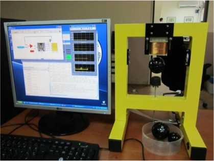
Fig. 1: Magnetic levitation system

F = mg - K_f

where m - is steel ball mass, ^g - gravitation constant, ^{K f} - magnetic force constant which is valid for pair electromagnet - ball, ⁱ - current which flows through electromagnet, x - ball distance from magnet. Using second Newton’s law, equation (4) can be rewritten as:

m^x = mg -к dt2              f

One of its magnet poles is pointing to the middle part of frame. Sensor for tracking ball position is installed in wall of the middle frame part. Ball holder (where the ball is positioned when system is inactive) is installed on bottom part of the frame. There are also magnetic levitators with two electromagnetic coils and in that case, instead of ball holder, second electromagnetic coil is installed. In this paper we used magnetic levitation system [7] with one electromagnetic coil (Fig. 1), so the second type of levitation system will not be described further.

Magnetic levitator can be divided into two subsystems, mechanical and electrical [8]-[10]. For electrical subsystem it is important to single out electromagnetic coil inductance (^^ and its resistance Rl ⁽^) . Electrical subsystem can be described with the following well-known differential equation:

U = Ri + Ldi dt .                                       (1)

In order to determine the current in coil, the resistor ^{R S} is serial connected to the coil. In that way voltage ^{U S} can be measured across resistor ^{R S} , by using A/D convertor for measuring current i . Now, (1) rewritten as:

di

U = (R + Rs ) i + L —

.

After applying Laplace transform we obtain:

Ils!        1

e ()  V (s)  Ls + ( R, + Rs )

The value of electromagnetic coil current in steady state ^{i SS} can be determined by (5). That current defines constant of ball position ^{x SS} in a steady state. If we take into consideration that velocity and acceleration are equal to zero in steady state, i.e., dxldt = d x dt = 0, then (5) is given as:

i ^SS = mgx^

.

where I (s ) = Лi (t)] , U (S) = Лu (t)] ,

Laplace transform operator.

can be

^л is

On the other side, modelling mechanical subsystem can be performed simply by defining force F , that represents result of electromagnet activity to the ball:

Theoretically, regulation of the ball position can be performed by (6). Anyway, external disturbances, uncertainty and system parameter variations affect on existence of high nonlinearity degree and require feedback controller installation which purpose is advancement of mechanical subsystem performances. In general, adding linearity into the system must be done first [11], and after that control process begins. In this paper NARX neural network is used for experimental substitution of real system of magnetic levitation. If training process is successfully performed, we are going to get values on network outputs with minimal errors comparing to the real levitator output values. In that way authentic experimental work with simulator of magnetic levitation system can be provided only by programming in MATLAB software. Magnetic levitation system block diagram is shown in [7]. Nonlinear mathematical model of Inteco magnetic levitation system is given by the following equations:

F x 2 =- em + g, m

x. =---7(ku + c. - Хд ),

³     f. ( Х 1 ) ⁽ i i ³ )

2 ^F emP 1            ^x 1

Fem = X3  p exp I p    I, emP 2     V    emP 2 )

fi ( Х 1 ) = fF exp I- xT- 1 ,

where ^x 2 ^e ^ , x ^{3 e[} x ^{3 MIN ,2.38 ]} , ^{u e[} u MIN ^{,1 ]} . Values

of used parameters in (7) are given in Table I.

Table 1:  Parameters of nonlinear mathematical model

Parameter	Value	Unit
m	0.0571 (big ball)	[kg]
g	9.81	[m/s2]
F em	f ( x 1 , x 3 )	[N]
F emP 1	1.7521 x 10 - 2	[H]
F emP 2	5.8231 x 10 - 3	[m]
f'. ( ^ 1 )	f ( x 1 )	[1/s]
fiP 1	1.4142 X 10 - 4	[ms]
fiP 2	4.5626 x 10 - 3	[m]
c i	0.0243	[A]
ki	2.5165	[A]
x 3 MIN	0.03884	[A]
u MIN	0.00498

Nonlinear autoregressive network with external inputs is recurrent dynamical feedback network which connects defined network layers. NARX model is based on linear autoregressive model, used for modelling serial time sequences. Function that characterizes NARX model can be represented as [12]:

y (t ) = f

' y ( t - 1 ) , y ( t - 2, ) ..., y ( t - n y ) ,

^ u ( t - 1 ) , u ( t - 2 ) ,..., u ( t - n ) у

From (8) it can be concluded that the next (predicted)

output signal value y ⁽ t ) is obtained from the previous

output signal values

,...,

y ( t — n y

and the previous independent input signal values

(u (t-1),u (t -2),...,u (t -n ))                  , , u . NARX model can be

Variables FemP1 and FemP2 are electromagnetic force ffc       k values, variables  iP1 , iP2 ,   i and i are actuator values, and variables x3MIN and uMIN are limitations.

implemented by neural network using conventional feedbacks for function f approximation, exclusively for making connections between output network vector y ⁽ t ) and inputs into layer 1. The block diagram of NARX neural network is shown in Fig. 2.

Inputs                   Layer 1                                   Layer 2

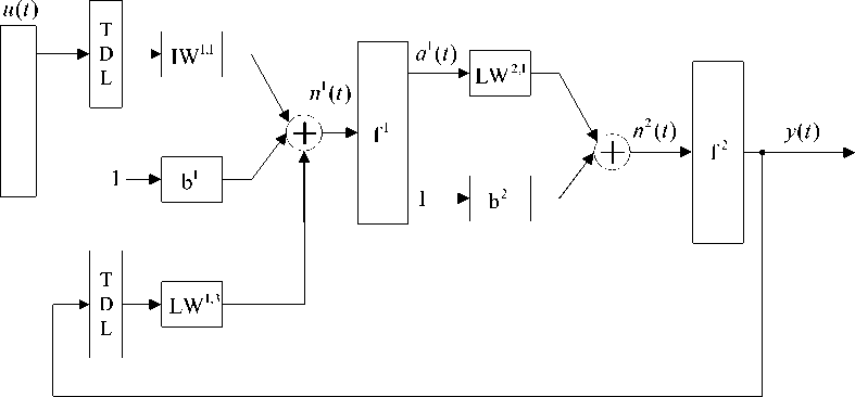
Fig. 2: NARX neural network block diagram

t u ( ¹ )

Vector

is brought to the system as two-layer input, passing through time delay block (TDL) and in that     way     part      of     function      (8),

( u ( t - 1 ) , u ( t - 2 ) ,..., u ( t - n„ ) )

u , is realized. Vector n (t)    is obtained from defined weight coefficients IW , , bias b , and output network vector

y(t) which is led to time delay block and after that multiplied by weight coefficients LW ,  . Obtained n1 (t) vector f1 function

is then led to the first layer activation . Output from the first layer a (t) , f1 representing action result of activation function , comes to the second layer where it is being transformed

(by weight coefficients ^{LW 2,1} treatment and bias ^{b 2} )

into vector

n2 (t)

This vector has been brought then on

f ²

bias     of input function and final neural network

output y ⁽ t )

is obtained after that. Output vector

У(t)

represents result of neural network working process,

and as we mentioned before, output vector is brought to TDL of layer 1.

That way the second part of depending function (8):

(u (t-1), u (t - 2)

.,u (t- nu ))

is realized. Described

model can be used as a predictor for the prediction of next input signal. It can be also used as nonlinear filter and in that case undesirable noises from input signals are removed.

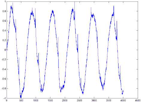
Fig. 5: Ball position changes with discretization period of

T = 0.25ms

• IV.    Neural Network Training Methods

Real data obtained from magnetic levitation system (explained in Section II) is used for training process. Current values from electromagnetic coil of magnetic levitator are chosen for training process input data, as well as position values (positions which steel ball have had at individual moments of time). Figures 4 and 5 represent levitation characteristics during PID control of ball position. Position and current values are taken with discretization period of ^T = 0 ^.25ms . Magnetic coil should be supplied with constant current (approximately 0.78A) in ideal case of ball levitation (levitation without oscillations). In Fig. 4, value 0.78A is zero position on vertical axis.

Current is changing in interval [-1, 1] during oscillations, which corresponds to the real values given in [A] in interval [0.77, 0.79]. That means that notch between 0 and 1 is making current changes up to 0.01A maximum. In Fig. 5, zero position on vertical axis represents ideal ball position if there are no oscillations.

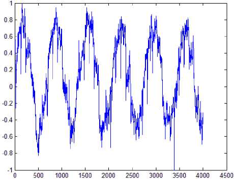
Fig. 4: Current changes with discretization period of T 0.25ms

Ball positions during work of levitation system are maximally changing 2.25mm comparing to ideal (zero) positions. That means that notch between 0 and 1 on vertical axis represents position change, which in maximal case (when position 1 is achieved) is 2.55mm.

After current and position data transformations into input and output vectors respectively, important parameters of future neural network are going to be defined. NARX neural network presented in previous section is chosen for modelling neural network. Eleven different training types [13]-[16] were applied on this neural network during realisation of experiments, and next three types of numerical optimization techniques were chosen:

• •    Conjugate gradient algorithms (Backpropagation method with Fletcher – Reevs type of parameters update, Backpropagation method with Polak – Ribieres updating type, Backpropagation method with Powel – Beales type of data reinitialisation, and scaled conjugate gradient method) [17],

• •    Quasi - Newton method (one-step interception method and basic Quasi – Newton type of updating parameters) [18],

• •    Levenberg - Marquardt method (method of Bayesian regularization, and basic form of Levenberg – Marquardt method) [19].

In addition of optimization techniques, basic methods of descending gradient are applied, as well as flexible backpropagation learning algorithm. Every mentioned type of training was tuned during experiment: neuron number modifications in hidden layers were done, as well as iteration number modifications during training process.

After completing dozens of experiments it is shown that best experimental results are obtained from two methods: basic Quasi – Newton type of parameters updating and Backpropagation method with Polak – Ribiere type of updating parameters. It is verified that those two training procedures can be used for simulating highly nonlinear systems and in next section obtained experimental results will be shown.

• V.    Experimental Results

  Basic Quasi – Newton method gives best results with 10 neurons in hidden layer. Training process achieved best performances after 2963 iterations. With further

increase of number of neurons in the hidden layer, network performances are improving slowly and it is estimated that optimal solution (if estimation parameters are number of neurons, training iterations and output values) is one with 10 neurons in hidden layer. Obtained results from this type of neural network, compared with results from real levitation system, are shown in Fig. 6.

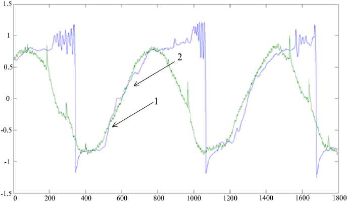
Fig. 6: Response of real (1) and simulated (2) system

Training type which obtained the best results from all experiments we have done is Backpropagation training method with Polak – Ribieres way of updating data. It is shown that for realization of this NARX network 20 neurons are optimal for implementation of hidden layer.

This network is achieving maximal performances after only 243 training process iterations, what is 12 times less comparing to Basic Quasi – Newton method. Obtained results from this type of neural network and results from real levitation system are shown in Fig. 7.

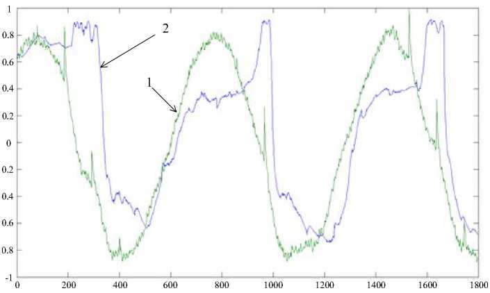
Fig. 7: Response of real (1) and simulated (2) system

Deviation graphs of two represented learning algorithms are shown in Figs. 8 and 9. It is considered that zero positions (on vertical axes) are values obtained from real magnetic levitation system. Results are showing that errors which occur are less than 1mm during whole simulation process which can be considered as good experimental results.

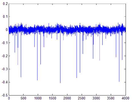
Fig. 8: Network deviations for Quasi – Newton training method

obtaining better results comparing to other training types mentioned in this paper are also represented. Nonlinear autoregressive network can be successfully used in complex systems, high nonlinear systems, systems where predictive neural network performances can be expressed.

The paper presented here was supported by the Serbian Ministry of Education, Science and Technological Development (projects III 43007, III 44006 and TR 35005).

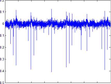
О 500    1000   1500   2000   2500   3000   3500   4000

Fig. 9: Network deviations for Backpropagation training method

Based on experimental results, we can conclude that NARX neural network (with appropriate training process and optimal number of neurons in the hidden layer) can simulate real magnetic levitator adequately enough. In this specific case, system response is shown as the change of the ball position regarding to the current which is powering electromagnetic coil. Voltages on coil and ball velocity during levitation process could be also used as experimental parameters.

• VI.    Conclusion

• [1]    I. Ahmad and M. Akramjavaid. Nonlinear model and controller design for magnetic levitation system. Proceedings of 9^th International Conference on Signal Processing, Robotics and Automation, University of Cambridge, United Kingdom, February, 20.-22., 2010, pp. 324-328.

• [2]    G.K.M. Pedersen and Z. Yang. Multi-objective PID-controller tuning for a magnetic levitation system using NSGA-II. Proceedings of 8^th Annual Conference on Genetic and Evolutionary Computation, July, 8.-12.,   2006, Seattle,

  Washington, USA, pp. 1737-1744.

• [3]    A. Trisanto. PID controllers using neural network for multi-input multi-output magnetic levitation system. Electrican Journal Rekayasa dan Teknologi Elektro, Vol. 1, No. 1, pp. 63-68, 2007.

• [4]    M.Y Rafiqa, G Bugmannb, D.J Easterbrooka. Neural network design for engineering applications. Computers & Structures, Vol. 79, No. 17, pp. 1541–1552.

• [5]    M. Anthony and P.L. Bartlett. Neural Network Learning:  Theoretical Foundations. Cambridge

  University Press, 2009.

• [6]    M. Lairi and G. Bloch. A neural network with minimal structure for MagLev system modeling and control. IEEE International Symposium Intelligent Control/Intelligent Systems and Semiotics, Cambridge, MA, September, 15.-17., 1999, pp. 40-45.

• [7]    Inteco, The Magnetic Levitation System (MLS)-User’s Manual, Available at www.inteco.com.pl , 2011.

• [8]    V. Dolga and L. Dolga. Modelling and simulation of a magnetic levitation system. Fascicle of Management and Technological Engineering, pp. 1118-1124, 2007.

• [9]    C.-A. Dragoş, St. Preitl, R.-E.Precup, R.-G. Bulzan, E. M. Petriu, and J. K. Tar. Experiments in fuzzy

  control of a magnetic levitation system laboratory equipment. Proceedings of 8^th International Symposium on Intelligent Systems and Informatics, Subotica, Serbia, 2010, pp. 601-606.

• [10]    C.-A. Dragoş, St. Preitl, R.-E.Precup, and E. M. Petriu. Magnetic levitation system laboratorybased education in control engineering. Proceedings of 3^rd International Conference on Human System Interaction, Rzeszow, Poland, 2010, pp. 496-501.

• [11]    P. Šuster and A. Jadlovska. Modeling and control design of magnetic levitation system. Proceedings of 10^th International Symposium Applied Machine Intelligence and Informatics, Herl’any, Slovakia, January, 26.-28., 2012, pp. 295-299.

• [12]    M.H. Hudson, M.T. Hagan and H.B. Demuth. Neural network toolbox 7, User’s Guide, 2012.

• [13]    C. Voglis and I.E. Lagaris. A global optimization approach to neural network training. Neural, Parallel and Scientific Computations, Vol. 14, pp. 231-240, 2006.

• [14]    B. Wilamowski. Neural network architectures and learning algorithms. IEEE Industrial Electronics Magazines, Vol. 3, No. 4, pp. 56-63, 2009.

• [15]    C.-A. Dragos, R.-E. Precup, E. M. Petriu, M. L. Tomescu, St. Preitl, R.-C. David, and M.-B. Radac. 2-DOF PI-fuzzy controllers for a magnetic levitation system. Proceedings of 8^th International Conference on Informatics in Control, Automation and Robotics, Noordwijkerhout, Netherlands, Vol. 1, pp. 111-116.

• [16]    R.-C. David, C.-A. Dragos, R.-G. Bulzan, R.-E. Precup, E.M. Petriu and M.-B. Radac. An approach to fuzzy modeling of magnetic levitation systems. International Journal of Artificial Intelligence, Vol. 9, No. A12, pp. 1-18, 2012.

• [17]    N.M. Nawi, R.S. Ransing, and M.R. Ransing. An improved conjugate gradient based learning algorithm for back propagation neural networks. International Journal of Computational Intelligence, pp. 780-789, 2007

• [18]    C. Broyden. Quasi-Newton methods. in Numerical Methods for Unconstrained Minimization, Ed. W. Murray, Academic Press, New York, 1972, pp. 87106.

• [19]    A. Ranganathan, The Levenberg-Marquardt algorithm. Tutorial on LM Algorithm, 2004.

Dragan S. Antić received the BSc degree from the Faculty of Electronic Engineering, Niš, in 1987, and his MSc degree from the University of Niš, in 1991. He received the PhD degree from the University of Niš, in 1994. He is currently working as Full Professor in

Department of Control Systems at Faculty of Electronic Engineering. He is author and co-author more than 180 scientific papers of refereed journals and international/national conferences. His research interests include sliding mode control, nonlinear systems, modelling and simulation of dynamic systems, bond graphs, and orthogonal polynomials.

Miroslav B. Milovanović received the BSc degree from the Faculty of Electronic Engineering, Niš, in 2011. He is currently working as Teaching Associate in Department of Control Systems at Faculty of Electronic Engineering. He is author and co- author of 15 scientific papers of refereed journals and international/national conferences. His current research interests include process control and identification, and neural networks.

Saša S. Nikolić received the BSc degree from the Faculty of Electronic Engineering, Niš, in 2006. He is currently working as Teaching Assistant in Department of Control Systems at Faculty of Electronic Engineering. He is author and co- author more than 50 scientific papers of refereed journals and international/national conferences. His research interests include control systems theory, process control and identification, sliding mode control, and orthogonal systems.

Marko T. Milojković received the BSc degree from the Faculty of Electronic Engineering, Niš, in 2003, and MSc degree from the University of Niš, in 2008. He received the PhD degree from the University of Niš, in 2012. He is currently working as Assistant Professor in Department of

Control Systems at Faculty of Electronic Engineering. He is author and co-author more than 60 scientific papers of refereed journals and international/national conferences. His current research interests include the modelling and simulation of dynamic systems, sliding mode control, fuzzy control, and orthogonal systems.

Stanisa Lj. Perić received the BSc degree from the Faculty of Electronic Engineering, Niš, in 2009. He is currently working as Teaching Assistant in Department of Control Systems at Faculty of Electronic Engineering. He is author and coauthor more than 35 scientific papers of refereed journals and international/national conferences. His current research interests include sliding mode control, fuzzy control, control systems theory, genetic algorithms, and orthogonal polynomials.