Software Effort Estimation Using Grey Relational Analysis

Published Online May 2017 in MECS

Effort estimation is an important aspect of the software engineering projects. Software effort estimation is one of the most important processes in software project development to be performed ahead of programming the software projects [1]. The development of a project by any company starts by making a perfect analysis about the requirements of a project. For this, abstraction of previous projects or analogy approach is used [2]. The estimates typically become targets when the project proceeds to the stages of detailed planning and execution. Improper estimation can lead to a variety of problems for both software organization and user organization.

Two issues have been observed at the time of quoting the project in the presence of different organizations to handle the project. First one could be, in case of over estimation, the bidding organization may lose the project, because the competing software organizations has estimated more accurately and quoted lower. Second one, in case of under estimation, the software organization will make a loss and also delay the delivery of the software [3].

The problem with estimation is that the project manager has to quantify the cost, effort and delivery period before the completion of the design. As more information is available, estimates can be more accurate. Estimation suffers due to incomplete knowledge, lack of time and various competitive pressures that are directly or indirectly put over the developer to arrive at more acceptable estimates. This can be achieved by selecting an efficient method to estimate accurately. Deng. J [4], a novel approach such as Grey Relational Analysis (GRA) is proposed. We are using this approach to predict effort estimation.

In 1980, Grey Systems Theory was introduced by Professor Deng Ju-long from China. It was a novel method applicable to the study of unascertained problems with few data and/or poor information [4-7]. Grey Systems Theory (GST) works on unascertained systems with partially known and partially unknown information by drawing out valuable information by generating and developing the partially known information [7]. The generation of partially known information is practiced much in software industries where incomplete information is given initially for development. Grey relational analysis is one part of the grey system theory. GRA is used to find out projects that are similar to a new project and configure the similar parameters required to estimate the effort or cost of a project.

In grey relational analysis, grey relational grades (GRG) are used to describe and explain the relationship between the referential object and compared objects [4]. K. H. Hsia et., al [5] presented a linear normalization that involved three kinds of measurements to avoid distorting normalized data.

This paper has been organized as follows: Section 2 describes related literature and previous works, Section 3 introduces various software effort estimation models, Section 4 introduces the Grey Relational Analysis (GRA) model, Section 5 illustrates evaluation and experimental results of the proposed model and finally Section 6 presents conclusion and future work.

• II.    Related Work

Estimating the effort and cost is the prerequisite process of the software development before handling the projects. The goal of a Software Manager is to deliver the software product efficiently with high quality. He is responsible to estimate the effort and cost efficiently in advance.

Qinbao Song et., al [8] had proposed a novel approach of using Grey Relational Analysis of Grey System Theory to address. The feature subset selection and software effort prediction at an early stage of a software development process on two types of datasets.

Sun-Jen Huang et., al [9] combined GRA with Genetic algorithms to estimate the effort on different datasets. In their work, the appropriate weights of the weighted GRG for each effort driver were prefixed to improve the accuracies of the software effort estimates. Sun-Jen Huang et.,al [10] proposed FNN model showed better software effort estimates in view of the MMRE, Pred(0.25) and MdMRE evaluation criteria as compared to the traditional COCOMO and the classical artificial neural network approach. The results demonstrate that applying FNN method to the software effort estimation is a feasible approach to addressing the problem of uncertainty and vagueness existing in software effort drivers.

Chao-Jung Hsu et., al [11] has proposed 6 weighted methods in this paper namely, non weighted, distance based weight, correlative weight and many. They showed the weighted GRA performs better than the non-weighted GRA. Especially, the linearly weighted GRA greatly improves accuracy as compared with the other weighted methods. Chao-Jung Hsu et., al [12] proposed 6 weighted methods. By using four public datasets, the performance of weighted GRAs is validated by comparing them with other techniques and published results. Particularly, the linearly weighted GRA can mainly improve accuracy and reliability of estimates. From the viewpoint of software practitioners, because there is no universally applicable method in all cases, they may still need more than one method or simultaneously adopt a series of methods to make correct decisions. In summary, we can recommend that GRA is an alternative or applicable method for software effort estimation.

Mohammad Azzeh et., al [13] had proposed Fuzzy Grey Relational Analysis (FGRA) model that produced and encouraging results with lower MMRE, MdMRE and higher Pred(25) on five publicly available datasets when compared to three well known estimation models (CBR, ANN and MLR). E. Praynlin et., al [14], proposed neural network based method to predict the effort, and had analyzed the performance of using historic dataset of NASA. From the results it is confirmed that Back Propagation Network (BPN) is efficient in software cost estimation compared to Elman network.

M. Pauline et., al [15] developed an enhanced system that focuses on minimizing the effort by enhancing the adjustments made to the functional sizing techniques. This paper presents fuzzy classification techniques as a basis for constructing quality models. Empirical validation for software development effort multipliers of COCOMO II model is analyzed and the ratings for the cost drivers are defined.

In Srinivasa Rao T et., al [16] used a stochastic approach was developed to estimate the effort by using K-means clustering to divide the projects, then on the clustered data PSO and neural network techniques were used to predict the effort. Jin-Cherng Lin et., al [17] was used computing intelligence techniques that is, PSO on clustered data within three to four groups to estimate effort and resulted in minimum error rate.

Jin-Cherng Lin et al., [18] applied computing intelligence techniques to identify key factors of projects such as ANOVA and Pearson. After recognizing the key factors the projects were clustered through k-means clustering and finally software project effort has been estimated using particle swarm optimization (PSO). The experimental results in this paper show that precise software effort has been estimated using computing intelligence techniques. Farhad Soleimanian et., al [19] used a novel Particle Swarm Optimization (PSO) was used to estimate the effort on only Kemerer dataset and proved that the error rate shows minimum with this method on the mentioned dataset

Geeta Nagpal et., al [20] used Grey Relational Effort Analysis Technique using Robust Regression Methods (GREAT-RM) to estimate the effort on individual projects. The authors implemented different estimators of robust regression and combined with GRA to estimate the effort on different datasets.

B.Chakraborty et., al [21] used Fuzzy Bayesian Belief Network (FBBN) rather than classical intervals in the COCOMO-II has been proposed and examined. FBBN-COCOMO-II produced better estimation results than the COCOMO-II using evaluation criterion MMRE, PRED (25%) and PRED (10%).

N. Shivakumar et., al [22] examined the effort from algorithmic method and nonalgorithmic method and proved that adaptive neuro-fuzzy based estimation is more efficient than the algorithmic methods for the estimation process. The success of estimation depends upon the accuracy and stability of the method in various measures. They implemented fuzzy method on existing database then compared with Doty, Bailed and Halstead methods. Finally, they showed the minimum error rate with fuzzy method compare to other methods through experimental results.

Thamarai et., al [23] used Differential Evolution (DE) method to select the most relevant project from set of historical projects that are similar to the new project. They used Desharnais dataset and compared with existing methods to prove minimum error rate with the proposed method.

• III.    Software Effort Estimation Models

One of the most identified algorithmic models for software effort estimation is COCOMO. In this work standard COCOMO model is used to estimate the effort of particular project using the equation given below:

Effort = a * size b              (1)

Here a and b are factors to calibrate using past data for each development mode and size means size of the project is in KSLOC.

Here we had considered three types of projects such as organic mode, semidetached mode and embedded mode.

Table 1. COCOMO basic model factor values

Mode	a	B
Organic mode	2.4	1.05
Semidetached mode	3.0	1.12
Embedded mode	3.6	1.2

Various algorithmic models of software effort estimation are presented in the table below. These models are used by the software team to find out the effort estimation and control the software projects. These models were compared with various projects from different models of effort estimation used by the project manager in the execution of the project.

Table 2. Various algorithmic models to effort estimation

Model	Equation	Factor a	Factor b
Halstead	Effort = a * sizeb	5.2	1.50
BaileyBasil	Effort = 5.5 + ( a * size b )	0.73	1.16
Doty	Effort = a * sizeb	5.288	1.047
Watson and Felix	Effort = a * size	5.2	0.91

• IV.    Methodology

In this work, Grey Relational Analysis is used to improve the quality of the project while the GRA provides the grades or ranks for the projects. This paper aims in producing better estimation of the cost and effort for a given project. The process of obtaining this approach is explained in the following sub-sections.

• A.    Grey Relational Analysis (GRA)

Grey system theory was proposed by Deng in 1980 [4]. From the Grey system theory (GST), Grey Relational Analysis (GRA) is a widely used method for analyzing a system in which the model is uncertain or incomplete information implying a combination of known and unknown information [6]. Grey Relational Analysis (GRA) also provides an efficient solution to complicated interrelationships among multiple response parameters.

Based on the Grey theory, a system can be investigated by means of Grey Relational Coefficient (GRC), Grey Relational Grade (GRG) so as to take final decision regarding selection of optimum variable combination based on highest grade i.e Grey Relational Ranking (GRR). The GRA is very effective to evaluate the multiple response parameters by converting individual response to a single GRG.

• 1)    Normalization

The first step is the standardization of the various attributes considered as duration, KSLOC and function points since they influence the effort estimation. In this paper, to normalize the parameters used, larger-the-better and smaller-the- better were used as shown in equations (2) and (3). The normalized values are always between 0 to 1.

Upper-bound effectiveness (i.e., larger – the – better):

• X: (k) - min X: (k)

x i ( k ) =---—-------(2)

max xt (k) - min xt (k)

Here i = 1,2, , , , m and k = 1,2,3, , , , n

Lower-bound effectiveness (i.e, smaller – the – better):

x_i ( k )^*

min X (k) - X (k) max X (k) - min X (k)

Here i = 1,2, , , , m and k = 1,2,3, , , , n

Where, x ( k ) represents the value of the k ^th attribute in the i ^th series;

*

• x ( k ) represents the modified grey relational generating of the k ^th attribute in the i ^th series;

maxx (k) represents the maximum of the kth attribute in all series;

min x ( k ) represents the minimum of the k ^th attribute in all series;

• 2)    Grey Relational Coefficient (GRC)

GRA uses the grey relational coefficient to describe the trend relationship between an objective series and a reference series at a given point in a system.

To calculate coefficients of parameters in all projects, Equation (4) was used.

GRC can be calculated as,

/ ( x o ⁽ к ), x ⁽ к » =

A min + Z A max

A_fi-№ + ZA 0 i            max

Here Z is the distinguishing coefficient. Generally, the distinguishing coefficient can be adjusted to fit the practical requirements.

Z G (0,1] i.e 0.5

Δ 0 i ( k ) =I x ₀ ( k ) - x_i ( k ) I   i.e. Delta values or

Deviation coefficients

Δ _min = min _i min _j I x ₀ ( k ), x_i ( k ) I

Δ _min = max _i max _j I x ₀ ( k ), x_i ( k ) I

• 3)    Grey Relational Grade (GRG)

GRG is used to describe and explain the relation between two sets. GRG can be used to show the degree of similarity between the project to be estimated and its historical projects. The greater the GRG between two projects, the closer relationship between these projects is [9].

1 ⁿ

Γ ( x ₀ ( k ), x_i ( k )) =   ∑ γ ( x ₀ ( k ), x_i ( k ))     (5)

ⁿ k = 1

Where, i ϵ {1, 2, 3, , , n} n is the number of response parameters

• 4)    Grey Relational Rank (GRR)

For the project to be estimated, the estimated effort should be retrieved from the historical data of project with the largest weighted GRG among all projects [9]. Ranks should be assigned with respect to the GRG with most influenced project to find effort estimation of new project.

• B.    Effort Prediction by Using GRA

To calculate the estimated effort of particular project with most influence k projects data, the following equation is applied [9].

n

ε ˆ = ∑ w_i * ε _i                (6)

i = 1

Where,

• ε ˆ is the predicted effort

• ε is the actual effort of influenced project

• w is weight is calculated by

Γ ( x , x )

w i = _k ^{0 i}                   (7)

∑ Γ ( x 0 , x i )

i = 1

Where,

Γ ( x , x ) is the GRG value of most influenced project i=1 to k means most k influenced projects

• V.    Experimental Results

In this paper, Kemerer dataset (Table 3) is used for evaluation and respective results are tabulated. On Kemerer data we applied GRA method to find the effort estimation and show the minimum error rate. The step by step evaluation of the proposed methodology is described as follows.

The process of estimating effort of first project is described below; same procedure is applied to every project to estimate the effort using GRA. Finally after estimate the effort of every project the error rate is calculated then show the minimum error rate.

Table 3. Kemerer data set

Project No	KSLOC	Actual Effort
1	253.6	287
2	40.5	82.5
3	450	1107.31
4	214.4	86.9
5	449.9	336.3
6	50	84
7	43	23.2
8	200	130.3
9	289	116
10	39	72
11	254.2	258.7
12	128.6	230.7
13	161.4	157
14	164.8	246.9
15	60.2	69.9

Step 1: Normalize the dataset: The whole data is taken as normalized values using Equation (2) as shown in the table below. The normalized values should be between 0 and 1.

Table 4. Normalization values

Duration	KSLOC	AdjFP	RAWFP	Effort
0.461538	0.522141	0.50623	0.417467	0.243333
0.076923	0.00365	0.184603	0.164609	0.054699
0.384615	1	1	1	1
0.5	0.426764	0.312021	0.358482	0.058758
0.307692	0.999757	0.560832	0.67947	0.288808
0	0.026764	0.145634	0.143576	0.056083
0	0.009732	0	0	0
0.230769	0.391727	0.404685	0.41198	0.098791
0.346154	0.608273	0.676515	0.666209	0.0856
0	0	0.063483	0.069959	0.045014
0.307692	0.523601	0.684716	0.688615	0.217229
1	0.218005	0.312248	0.286694	0.191401
0.576923	0.29781	0.267796	0.278006	0.123419
0.807692	0.306083	0.565318	0.584362	0.206344
0.346154	0.051582	0.427931	0.40192	0.043077

Step 2: Grey coefficient values can be found using    Equation (4) is used to find the similar projects from the

Equation (4) that helps to estimate the effort of the first    historical data.

project. To estimate the effort on particular project,

Table 5. Grey coefficient values

Duration	KSLOC	AdjFP	RAWFP	Effort
0.497797	0.423487	0.542593	0.601709	0.669869
0.834242	0.443585	0.435492	0.395262	0.33462
0.911223	0.801742	0.663346	0.86846	0.674699
0.713657	0.443711	0.877252	0.593116	0.896144
0.452205	0.434691	0.513978	0.582305	0.671508
0.452205	0.426379	0.429357	0.477247	0.610928
0.62353	0.746527	0.791438	0.989508	0.726355
0.769253	0.817701	0.692273	0.605658	0.708483
0.452205	0.421771	0.462553	0.523246	0.658618
0.713657	1	0.682077	0.584765	0.939066
0.414262	0.556499	0.663609	0.746	0.882696
0.769251	0.630191	0.615781	0.733484	0.762259
0.524224	0.638962	0.868256	0.696577	0.914455
0.769253	0.447399	0.831726	0.964236	0.656413

Step 3: Assigned the Grey Relational Grades (GRG) using Equation (5) to every project to estimate the effort of a particular project.

Table 6. Grey relational grades

Project No	GRG	Project No	GRG
2	0.547091	9	0.718674
3	0.48864	10	0.503679
4	0.783894	11	0.783913
5	0.704776	12	0.652613
6	0.530937	13	0.702193
7	0.479223	14	0.728495
8	0.775472	15	0.733805

. \

к          /      \          \               -«-GRG

05                          К

2 3 4 5 6 7 8 9 10 И 12 13 14 15

Project Number

Fig.1. Grey relational grades of evry project

The above figure shows the grey relational grades of every project. The grey relational grade is used to optimize the similar projects of reference project. Here reference project means current project is to be estimated effort.

Step 4: From the values of grey relational grades, assigned the ranks to every project as shown in Table 7. Here, only k influence projects from the ranking projects were taken to find the estimate the effort of a particular project.

Table 7. Grey relational ranks

Rank No	Project No	GRG	Rank No	Project No	GRG
1	11	0.783913	8	13	0.702193
2	4	0.783894	9	12	0.652613
3	8	0.775472	10	2	0.547091
4	15	0.733805	11	6	0.530937
5	14	0.728495	12	10	0.503679
6	9	0.718674	13	3	0.48864
7	5	0.704776	14	7	0.479223

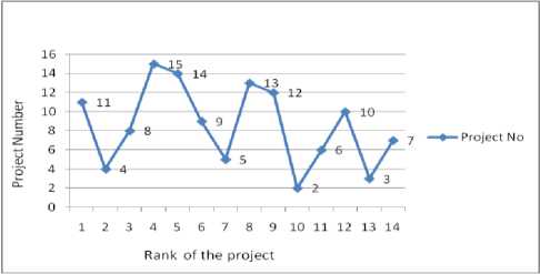
Fig.2. Grey relational ranks of every project

The above figure shows the grey relational rank of every project from grey relational grades.

Step 5: Predicted the effort of a particular project using Equation (6). From the grey relational grades, most influenced projects are to be considered with highest GRR values. Using GRG values, it was found the estimated effort of a particular project as shown below.

For example k most influenced projects of current project i.e. predict the effort of the first project. Here we are selected k=5, from Table 7 select first five projects GRG’s. Calculate weight from those GRG’s.as shown in below Table 8.

, =  Г( x 0, x, )

i       k

ЕГ( x o, xi)

i = 1

Here Г(xo, xt) is the GRG value of most influenced project k =5 i.e most k influenced projects

Table 8. Estimated effort using proposed method

Influenced Project No	GRG of influence d project	Weights	Actual effort of influence d project	Weight * Actual effort of influenced project
11	0.783913	0.2059905	258.7	53.289734
4	0.783894	0.2059855	86.9	17.900138
8	0.775472	0.2037724	130.3	26.551545
15	0.733805	0.1928235	69.9	13.478362
14	0.728495	0.1914282	246.9	47.263614
Sum	3.805579			158.48339

This process can be repeated to every project using the proposed method. Estimated effort of every project is shown below Table 9.

Table 9. Estimated effort using proposed method

Project ID	Actual Effort	Estimated Effort using proposed method
1	287	158.4833872
2	82.5	79.3454572
3	1107.31	219.9509304
4	86.9	174.169513
5	336.3	208.6745154
6	84	78.16597002
7	23.2	90.04539176
8	130.3	142.4321141
9	116	220.0229945
10	72	79.40079255
11	258.7	222.8425189
12	230.7	139.4482826
13	157	152.5512605
14	246.9	253.375697
15	69.9	133.7888356

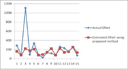
Fig.3. Comparison between actual and estimated effort using proposed method

The above figure shows the actual effort and estimated effort of every project. Most of the projects show the better effort then actual effort. The results obtained from the proposed model proved its efficiency.

The experimental results of the proposed method can be compared to that of the existing results on same dataset as shown in the Table 10.

Table 10. Comparison various models of effort estimation to the proposed model

Project No	Size in KSLOC	Actual Effort	COCOMO Estimate	Halstead Estimate	BaileyBasil Estimate	Doty Estimate	Watson and Felix Estimate	PSO Estimate	Proposed Estimate
1	253.6	287	802.73	21000.38	454.38	1739.54	801.27	284.03	158.483
2	40.5	82.5	116.96	1340.25	58.95	254.85	150.93	44.24	79.345
3	450	1107.31	1465.83	49638.9	878.57	3171.06	1350.28	507.97	219.95
4	214.4	86.9	672.97	16324.52	374.93	1459.09	687.72	239.58	174.169
5	449.9	336.3	1465.49	49622.35	878.34	3170.32	1350.01	507.85	208.674
6	50	84	145.93	1838.48	73.75	317.77	182.83	54.77	78.165
7	43	23.2	124.55	1466.24	62.79	271.35	159.38	47.00	90.045
8	200	130.3	625.59	14707.82	346.31	1356.65	645.56	223.27	142.432
9	289	116	920.78	25547.6	527.85	1994.58	902.44	324.26	220.022
10	39	72	112.42	1266.49	56.66	244.98	145.83	42.58	79.4
11	254.2	258.7	804.72	21074.96	455.61	1743.85	802.99	284.71	222.842
12	128.6	230.7	393.47	7583.41	209.69	854.41	431.92	142.70	139.448
13	161.4	157	499.47	10662.49	271.26	1083.84	531.12	179.65	152.551
14	164.8	246.9	510.52	11001.18	277.76	1107.75	541.29	183.49	253.375
15	60.2	69.9	177.33	2428.84	90.15	385.94	216.48	66.11	133.788

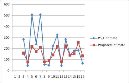
Fig.4. Comparison of PSO estimate with proposed estimate

The above figure shows the estimated effort using PSO and proposed model. Our proposed model was proved better results than PSO estimate. When we compare proposed estimate with other models, then prove the better results with proposed model as shown in Table 10.

From the above experimental results it is clear that the proposed model estimated effort is very close to the actual model. Experimental results also show the comparing results obtained after comparing the proposed model with Mean Magnitude Relative Error (MMRE) factor.

n

mere = — Mere N £

Here N means number of projects and MRE means Magnitude Relative Error which is calculated as follows ere =

|ActualEffo rt; - EstimatedEfort _t 1 ActualEffo rt

The comparison of the efficiency of the proposed model with various algorithmic models is mentioned in the Table (10).

With the proposed estimate of every project calculate MMRE using Equation (8). Proposed model shows the minimum error rate with other models as shown in Table 11.

Table 11. Comparison of efficiency of the various models with proposed model

Model Name	MMRE(%)
COCOMO	244.2667
Halstead	7679.953
Bailey-Basil	101.5933
Doty	647.12
Watson and Felix	268.0933
PSO	56.74026
Proposed model	54.78

The results of the proposed model gives a better estimation compared to the various algorithmic models of effort estimation and shows as minimum error rate as desired in above table and the same is depicted clearly in the below figure.

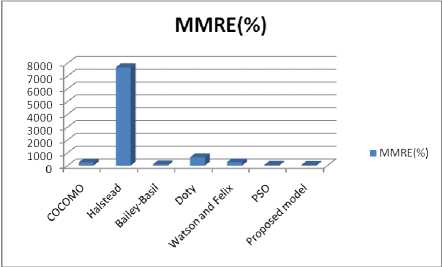
Fig.5. Efficiency of MMRE is comparison of various models with proposed model

Through the experimental results, from the point of MMRE, the proposed model is proven to be more efficient in comparison to the various models in terms of accuracy in estimation resulted in better performance.

• VI.    Conclusion And Future Work

Software projects development is a very challenging task to be handled by any industry. Effort estimation for the developing projects has to be predicted before the actual software development, in such way that the newly developed project must exhibit higher quality in less cost. To accomplish this, project management team must select a best model to achieve the mentioned goals and deliver the project in time. This paper states that in order to model a project, accurate and reliable effort estimation is required with respect to the project conditions. Achieving this goal needs accurate and reliable effort estimation and takes the place according to the project conditions.

In this paper, the proposed model uses Grey Relational Analysis (GRA) to estimate the effort of particular project, and experimental results show minimum error rate when compared to other algorithmic models of effort estimation.

Further extension of this work can be done by combining the proposed model with other techniques including other effort adjustment factors on different datasets.