Software for Simulating Neural Network Workload Impact on Mobile Devices

Recent advancements in CPU and GPU architectures allow mobile devices to efficiently perform complex operations, including machine learning model inference and, more recently, on-device model personalisation and training [1]. The new window of possibilities means our devices will be used more frequently for battery-draining tasks, such as training neural network models. Currently, such heavy operations are restricted to occur only when the device is charging, idle, sufficiently charged, and connected to a metered network. It ensures that the user has a minimum impact from these background loads [2]. However, this "safe" scheduling approach limits domains that require fast reaction times (e.g., glucose level prediction models and federated learning), forcing operations to be delayed to specific windows much later in the day.

We need to develop and compare new algorithms to find an optimal scheduling approach - one that minimises user interference while maximising training opportunities. When a mobile device is on, it has a constantly changing state. Even with the screen off, background or foreground activity consumes resources. A mobile device state is defined by a vector of eight connected variables, including battery, performance, screen, and thermal metrics. These factors influence each other; user actions, such as launching heavy apps or increasing brightness, automatically trigger chain reactions in power consumption and device thermals [3-4].

The goal is to minimise impact on the user device experience while maximising the number of windows (opportunities) for training [5]. Validating the scheduling algorithm [6] that would achieve this requires comparing it against others on the same vector of device states over time. It is impossible to achieve manually. Running the same test multiple times is unreliable due to external factors like ambient temperature, battery health degradation, and internal kernel processes. Even automated testing frameworks cannot control these stochastic variables. Furthermore, relying on real-time hardware testing is unscalable; a slight change in an algorithm might require a complete 24-hour rerun to verify. It creates a need for a software solution that utilises real mobile data samples to repeatedly run tests, achieving a close-to-real-world simulation of device states with heavy workloads overlaid at specific intervals.

2.    Related works

The feasibility of running heavy neural network training directly on mobile devices has been a significant focus of recent research. In [7], the authors surveyed the current landscape, noting that training locally is crucial for user privacy and personalisation. However, simply running these models isn't enough; we need to know the cost. In [8], the research tackled this by measuring training performance across various Android phones and providing a detailed breakdown of the energy, memory, and thermal costs involved. Authors in [9] further emphasised this by highlighting a critical constraint. These heavy workloads cannot come at the expense of the user experience, such as causing app lag or draining the battery unexpectedly. To manage these costs, several teams have proposed intelligent scheduling systems. For instance, authors in [10] developed a decentralised scheduler that uses reinforcement learning to balance deep learning tasks across different processors, achieving notable energy savings. The paper focuses on solving the problem of dynamic configuration for multiple concurrent neural network consumers competing for resources, but it does not account for the timing of executing these workloads. Given that the main objective is to maximise resource utilisation and that the approach is decentralised, the problem of improving the user experience remains. Another uncertainty lies in the test results reported in the paper, which are obtained by performing physical tests on real devices. Such test scenarios cannot be accurately rerun multiple times with different settings to demonstrate the impact of different configurations.

Another study [11] focused on thermal management, developing a system that dynamically switches tasks between the GPU and a low-power NPU to prevent overheating. Similarly, work [12] employed a combination of deep learning and integer programming to minimise battery current fluctuations, thereby extending battery life by approximately 7-8% in their tests. These papers reveal the problem of the time-consuming and non-deterministic nature of running the same experiment multiple times on a real device. Moreover, the results are obtained from a single device, and the developed scheduling approaches cannot be easily shown to be as effective on other devices.

More recent research into energy-aware federated learning [13] specifically calls for the development of standardised benchmarking tools that evaluate not just accuracy, but also energy usage, scalability, robustness, and privacy trade-offs – something that repeatedly testing numerous scenarios on a real device cannot achieve effectively. Another study on inference coordination [14] notes that device RAM must be shared between the OS and intensive AI tasks, making deterministic testing on physical hardware nearly impossible. Lastly, the benchmarking solution developed from the research [15] aggregates valuable data on the energy costs of different neural network workloads across selected physical devices, but it does not provide an environment to investigate and fix the scheduling problems it identifies.

Therefore, proving the effectiveness of the developed schedulers and optimisation attempts remains a challenge. To address this problem for high-level cluster schedulers, researchers have developed trace-driven simulators, such as DewSim, which replay Android device logs to simulate mobile clusters [16]. The same group later expanded this with an IoT testbed to automate benchmarks on physical phones [17]. However, the software proposed in their research is cluster-oriented. It treats the mobile (IoT) device as a monolithic node, meaning it does not capture resource contention within the device or thermal-aware performance fluctuations. While these tools are excellent for studying distributed workloads across a cluster of devices, they are less suited for deep, single-device investigations.

The academic community is facing a reliability crisis due to high signal-to-noise ratios, low repeatability, and non-deterministic results in physical device testing. The existing tools do not provide a granular, controllable and repeatable way of simulating neural network workloads over existing system traces, meaning there is still a gap for a platform that can accurately simulate the complex, moment-to-moment thermal, power and memory impacts of neural network operations (and other heavy workloads) on mobile device traces. The focus of this work is to bridge this gap by providing a simulation platform that opens up possibilities for further research into optimising scheduling algorithms.

3.    Methods and Materials

A vector of the following sub-states can represent a generalised mobile device state:

• •   Battery level percentage;

• •   Battery Voltage;

• •   Battery Current;

• •   CPU activity percentage;

• •    Memory usage percentage;

• •    Screen state (on/off);

• •   Screen brightness percentage;

• •    Thermal indicator.

Some of these states have a direct reactive relationship (e.g., higher screen brightness will produce more current, resulting in a drop in voltage, which in turn will cause a faster decrease in overall battery level, and, as a side effect, will also impact the thermal measurement). In contrast, others are triggered by user activity (e.g., the screen is on, high-intensity applications are launched, resulting in higher CPU activity and memory usage [18], as well as all the power implications).

We propose a mathematical model in which the simulation result is the product of a baseline device recording overlaid with the footprint of a resource-intensive task. The simulated output data is a vector of device states that mimics what the actual device recording would be like if that resource-intensive task had been executed at the given time in the baseline data.

CPU metric simulation model

This CPU simulation model overlays training-induced overhead onto a baseline CPU profile. The training overhead is the positive difference between the observed training CPU and a "workload baseline" calculated as the mean of the final N. To model saturation, this added overhead is adaptively reduced via exponential scaling when the system's baseline CPU is already high, preventing unrealistic values. Finally, Gaussian noise is added to introduce variability, and the total simulated CPU is clamped to 0-1 (0%-100%).

C_s(t) = clamp_[0 , _1](C_b(t) + s(t) ■ max(0,C_t(t) - C t ) + .W(0,a²)),

(t) =

( a + (1 - a) ■ exp

1,

(-k^(^.i)).

ifC_b(t) >  C_t. otherwise,

where C_s(t) - is the simulated CPU utilisation at time t;

C_b (t) - is the baseline CPU utilisation at time t;

C_t (t) - is the predicted value of the data point;

C_t - is the training CPU baseline, the mean of the last ^_tail samples; s(t) - is the dynamic scaling factor accounting for baseline saturation; a - is the asymptotic minimum scaling factor;

• к - is the exponential decay rate parameter;

^(0. a ² ) - is the Gaussian noise with variance a ² .

The saturation scaling factor s(t) is based on the Law of Diminishing Marginal Returns [19], which is relevant for the case, as when the multi-core device approaches full load, the capacity to process extra instruction cycles decreases in a nonlinear way (caused by the cache contention problem and the context switching overhead). That is why an exponential decay function is used to model the transition to a saturated state.

Thermal metric simulation model

The device thermal model [20] is based on a first-order lumped thermal Resistor-Capacitor model and balances two mechanisms: CPU-driven heat accumulation and, following Newton's Law of Cooling, passive dissipation [21-24].

Key parameters governing thermal sensitivity and cooling rate are learned from training data by correlating CPU and thermal changes. Post-training, thermal headroom is interpolated back to the baseline using either a learned cooldown rate or a fixed linear interpolation. During the simulation, the net rate of thermal headroom change is calculated by:

^ = a^ (C_s& - C_b(t)) - 0 ■ (T_s(t) - T_b&)),                        (2)

where T_s(t) - is the simulated thermal headroom;

T_b (t)- is the baseline thermal headroom;

a - is the thermal sensitivity coefficient (heating);

0 - is the thermal dissipation constant (cooling);

In the discrete-time simulation, the thermal state is updated iteratively:

Ts(t) = Ts(t - 1) + a ■ AC(t) - HTs(t- 1)- Tb(t - 1))                      (3)

where T_s(t) - is the simulated thermal headroom;

T_b(t)- is the baseline thermal headroom;

a - is the thermal sensitivity coefficient (heating);

0 - is the thermal dissipation constant (cooling);

After the training segment ends, the system naturally returns to the baseline state. The cooldown segment is modelled using an exponential decay function rather than linear interpolation (based on the physical principle of exponential dissipation):

T_s(t) = T b (t) + (T_end - T b (t_end)) ■ e—f^-t end)

where T_s(t) - is the simulated thermal headroom at time t

T_en d - is the thermal headroom when training ended;

tend - is the time when training ended;

0 - is the thermal dissipation constant (cooling);

Memory metric simulation model

The memory simulation uses a delta-based approach, applying training-induced memory changes to a baseline profile. The training memory baseline is calculated by averaging the initial and final N-sample means. The model is asymmetric: it only adds positive deltas to the system's baseline profile. If the delta is zero or negative, the baseline is used unchanged. It reflects that training allocates memory but cannot free the baseline system's memory.

ад) =

^clamP [o,i] [

M_b(t) + max(0, M_t(t) M b (t)

-M t )

if M_t(t)-M_t>0 otherwise

where M_s(t) - is the simulated memory utilisation at time t;

M_b(t) - is the baseline memory utilisation at time t;

M_t(t) - is the measured training memory at time t;

M_t - is the training memory baseline, average of first and last ^_init samples.

Power consumption metric simulation model

The developed power consumption model relates CPU utilisation to power draw using a piecewise polynomial regression [16-17]. The model partitions the CPU utilisation range into three segments, characterised by linear (low), quadratic (mid), and cubic (high) scaling. This piecewise approach is necessary to capture the fundamentally nonlinear relationship between CPU load and power, which is influenced by factors such as dynamic voltage/frequency scaling and thermal throttling. Power is computed from measured current and voltage. The model is trained on training data and calibration data (optional), where the latter is filtered by charging state (charging or discharging) to ensure consistency with the training data.

The piecewise power prediction function is:

(P low (C)  if Ce^

P(C)= P mid (C)  if ce^ mid

Phigh(C)  if ce^high where P(C) - is the predicted power consumption for CPU utilisation C;

C - is the CPU utilisation.

The battery current simulation translates CPU-driven power changes into current draw, applying only during discharging states, as charging current is not dictated by device load. The simulation computes the power differential between the simulated and baseline CPU states (using the piecewise power model) and converts this power increase to current using the instantaneous battery voltage. A clamped voltage correction factor is applied to account for discrepancies between the simulation voltage and the model's training reference. The model is asymmetric, applying only positive CPU deltas (increased load) to the baseline current, since decreased load does not reduce consumption by other system components.

When the CPU delta is positive, and the device is discharging, the power increase is calculated:

bP(t) = P(C_s(t»-P(C b (tV,                                 (7)

where ^P(t) - is the power increase at time t;

P(C_s(ty) - is the predicted power at the simulated CPU;

P(C_b(ty) - is the predicted power at baseline CPU.

The voltage simulation model applies the voltage pattern from the training data, calculated as changes relative to the initial training voltage, onto the baseline's starting voltage, indexing the pattern by elapsed simulation time. A simplified, current-driven fallback model that calculates voltage sag based on internal resistance is used only when training voltage data is insufficient. This simulation is turned off during charging states, as the charging circuit then controls the voltage.

The voltage deltas from training data are extracted as:

• V _t(t_t) - is the training voltage at time t_t ;

V_t (t₀) - is the initial training voltage;

• ^ _t - is the number of training samples;

The simulated voltage using the delta-based approach is:

K(t)=K tart +

where K(t) - is the simulated voltage at time t;

Kurt- is the baseline voltage at training start;

8_v[j (t)] - is the voltage delta at training index j (t);

This battery level simulation employs a linear drain model, utilising a constant consumption rate derived from the training data (total battery loss divided by the training duration). This rate is applied progressively during the training window, and the final cumulative loss is maintained persistently after training ends. The model is asymmetric: charging pauses the simulation, using the baseline level. If the baseline recharges past the battery level observed at the end of training, the cumulative loss is cleared to reflect recovery.

The battery drain rate is computed from training data:

ra

^ t C^ end )  ^ t^(t start )

S train         ,

where r_d - is the battery drain rate per second; P_t(t_end) - is the battery level at the training end; P_t(t_start) - is the battery level at training start; Ptram - is the training duration;

The simulated battery level is calculated differently depending on context:

(B_b(t),                if charging,

B_s (t) = \ B_b (t) + r_d ■ t elapsed , if in the training window and discharging, B_b (t) — AB_total,      if after training and discharging,

where B_s(t) - is the simulated battery level at time t;

B_b (t) - is the baseline battery level at time t;

• r _d - is the drain rate per second;

• t _elapsed — is the time elapsed since the training started;

ABtotal - is the total cumulative drain.

Software architecture

The framework utilises a distributed architecture comprising an Android-based data collection layer and a Pythonbased analysis workstation.

The Android device serves as the testbed, hosting the applications that generate stress, running the training operations, and recording the device's state.

A background service application called Device State Collector monitors system APIs (BatteryManager, ActivityManager, Thermal Service) and serialises state vectors at 1 Hz.

A custom load-generation engine called StressLab, capable of synthesising CPU and memory pressure, is also installed on the device to help achieve specific stress levels.

The desktop workstation receives CSV telemetry via ADB for processing by the Python Emulator, which houses the mathematical models, simulation engine, and correlation analysers.

The distributed architecture enables recording to occur while the device is in a usable, non-paired state. So, the collector application is standalone and does not require a constant ADB connection.

Data acquisition is handled by a native Android application built using Kotlin and Jetpack Compose. To ensure measurement consistency and prevent the operating system from throttling the collector, the architecture relies on a Foreground Service with partial wake-lock acquisition.

The core component, DeviceStateMonitor, utilises Kotlin Coroutines to emit reactive streams of DeviceState objects. These objects contain a state vector:

• •    Battery – level (%), instantaneous current (mA), voltage (V), and charging status

• •    Memory – total, used, and available RAM (MB), including low-memory triggers

• •    Thermal – thermal headroom (normalised 0–1) and throttling status

• •    CPU – aggregate utilisation percentage

Data persistence is managed via the Room database (SQLite), ensuring session integrity before export.

Scheduling algorithm

Scheduling algorithm В

simulated recording of task overlayed over baseline at

'baseline' recording

(e.g. 24 hours)

Device State Collector (Android appt

provides timestamp В

produces

heavy task' recording

(eg. 15 minutes)

Input raw data

Simulator

•produces—> timestamp В

Simulated recording of Us к overlayed over baseline at

Fig. 1. The overall system architecture.

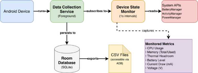
Fig. 2. Data flow architecture.

The CPU stress mechanism employs a multi-threaded architecture with one worker coroutine per physical core. To achieve load levels (e.g., 50% vs 100%), the engine utilises a time-sliced duty cycle within a 100ms window.

During the active phase, the system executes square root calculations in a tight loop. Results are checked against a sum to prevent compiler optimisations. Followed by the "idle" phase, threads sleep for the remainder of the window.

Simulating high memory pressure on Android is non-trivial due to the Dalvik/ART runtime's per-process heap limit (typically ~512MB on test devices). To circumvent this, StressLab implements a multi-process strategy. A MemoryServiceController dynamically spawns up to 30 isolated instances of MemoryEaterService, each running in its own OS process. Each service allocates ~250MB chunks using CharArray structures. The arrays are explicitly filled with data to force immediate physical page commitment, bypassing the OS's lazy allocation optimisation. The controller monitors total system RAM and adjusts the number of active processes to maintain the target saturation level.

The simulation engine is developed in Python 3.x, utilising NumPy and pandas for vectorised data manipulation. The power models (piecewise) are implemented using scikit-learn.

The interface is built with PyQt6, providing a GUI for managing experimental protocols, visualising real-time overlays via matplotlib, and executing automated correlation analyses.

4.    Experiment

The simulator's accuracy is crucial for future iterations of the developed system and for further research, as it will influence experimental results and ultimately determine the outcomes of scheduling algorithm comparisons.

Experiment methodology

The simulation's accuracy under realistic device conditions was assessed using a baseline-overlay methodology. This approach tests the hypothesis that complex device states can be modelled by superimposing isolated training overheads onto natural (recorded) dynamic system baselines.

Given the time-consuming nature of the experiments, a set of two devices was selected for this initial research phase. Based on the results and discussions, a larger set of 10+ devices (with different CPU and battery architectures, software optimisation) will be considered.

Multiple experimental scenarios were developed, and for each, data were captured across three distinct phases. For the baseline recording (phase 1), the natural system behaviour is captured (either idle or under external stress) without the presence of the training workload. It is followed by an isolated recording of the specific training operation (phase 2), which serves as the input for extracting the model's cost coefficients. The duration of the training operation was estimated by running and measuring a federated learning task over 10 epochs using the official "Flower" application. Finally, a complete recording of the entire experimental timeline (phase 3), which includes idle periods, induced stress, training workload, and recovery phases. The duration of the idle periods was chosen based on the device's experimentally derived cooldown period.

Apart from the experimental recordings, a 3-hour-long calibration segment was recorded for every device in the experiment. During this recording, the device was placed under various combinations of external and internal conditions, including processor load, screen brightness, idle cooldown periods and throttling conditions. This calibration model was then used for each experiment to aid with the power model, as described in the section above.

The validation pipeline consists of 5 steps. Firstly, high-resolution metrics (CPU, memory, thermal, battery, current, and voltage) are recorded at 1 Hz intervals on the target hardware. Next, the training-only segment is extracted to compute the resource baselines and overhead deltas.

Within the simulation step, the emulator inputs the baseline recording and mathematically superimposes the training effects to generate a simulated scenario. Next, the simulated scenario is compared with the ground truth, yielding 5 metrics: Pearson correlation, Mean Absolute Error (MAE), Raw Accuracy, Bias-Corrected (BC) Accuracy, and Concordance

Correlation Coefficient (CCC). The BC parameter is useful at this stage of development, as it accounts for potentially different signal starting positions.

This methodology isolates the emulator's ability to decouple training costs from environmental noise and accurately reapply them to varying system states.

• 1.    "Idle-Train-Idle" – the device is kept idle for 5 minutes, after which a training session is conducted, followed by a 5-minute idle period.

• 2.    "Idle-Load-Train-Idle" – the device is kept idle for 5 minutes, after which a stress load is applied to both CPU and memory, followed by a training session, followed by a 5-minute idle period.

• 3.    "Idle-Train-Screen-Idle" – the device is kept idle for 5 minutes, after which a training session is conducted with the screen turned on, followed by a 5-minute idle period.

• 4.    "Power-Idle-Load-Train-Idle" – same as "Idle-Load-Train-Idle", only during an active charging state.

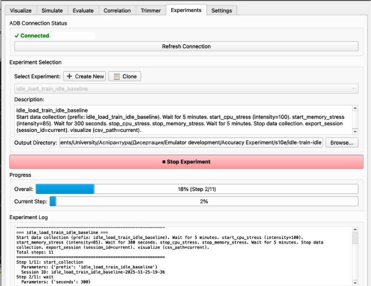
Fig. 3. Example of the "Experiment" tab UI during a running experiment.

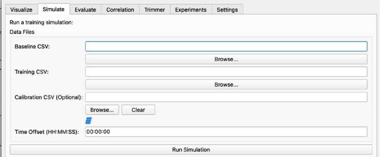
Fig. 4. Example of the "Simulate" tab, which allows for workload overlay simulation.

Experiment execution details

The "Experiment" tab, developed, enables users to select an experiment preset and run it automatically on a connected device via ADB. A preset consists of steps, such as starting device-state collection, running a stress or neural network training session, and exporting the resulting recording, among others. The progress of the experiment is illustrated, along with the current step's progress. This tab also allows the user to build a new experiment.

The experiment's functionality is designed to run entirely automatically. It utilises a wireless ADB connection to launch experiment steps without requiring manual user interaction with a display that is turned on (which consumes extra power and increases CPU load).

The simulation tab allows the user to apply an overlay of a heavy task recording (e.g., training a neural network) to the supplied baseline recording at a specific timestamp.

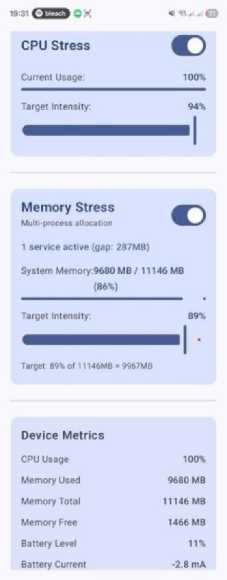
Using the accuracy test tab, the user can then compare the simulated recording to a "ground truth scenario" recording. And evaluate the accuracy. The tab lets you select the correlation algorithm and toggle simulated metrics on or off. The result displays the accuracy of each test and the overall accuracy, along with the parameters available in an exported report. Using the developed stress simulation application, users can adjust CPU and memory stress levels via ADB commands. It eliminates the need to interact with the user interface, allowing tests to run with the device screen off when necessary.

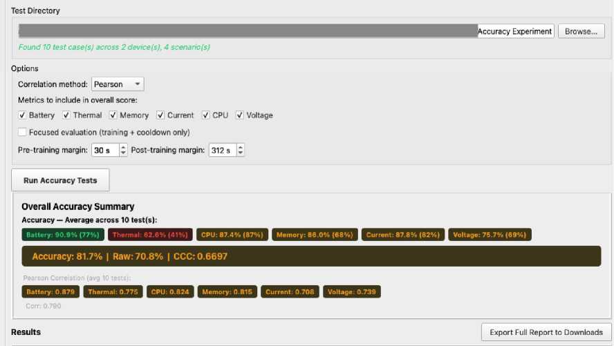
Fig. 5. Example of the accuracy tab UI with intermediate accuracy test results.

Device Metrics Collector

Data Collection Status

I Active

Start Collection

Stop Collection

Data Export

- Session ID--------------------- training_segment 2

025-11-12-15-38 V

The data collection service runs in the background and is designed to be unkillable It will automatically restart if terminated by the system.

Fig. 6. Screenshots from the StressLab application and the Device State Collector application.

Using the developed stress simulation application, users can adjust CPU and memory stress levels via ADB commands. It eliminates the need to interact with the user interface, allowing tests to run with the device screen off when necessary.

5.    Results

The image below illustrates a comparison between the simulated (colourful, solid charts) and the "ground truth scenario" recording (dashed grey charts).

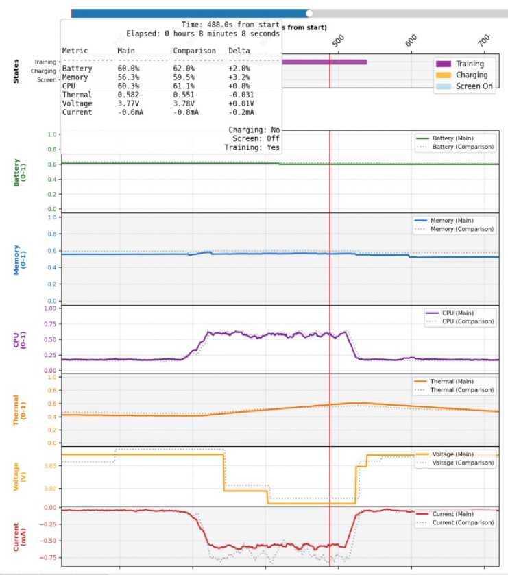
Fig. 7. Example of the visual comparison output for simulated vs "ground truth scenario" recordings.

Multiple test scenarios were run consecutively to verify the results on two test-subject devices. The experiments and their identifiers are listed in Section 4. For each signal, we compute the Root Mean Square Error (RMSE) and normalise it by the observed signal range to obtain NRMSE. The bias-corrected accuracy is also reported.

Table 1. Simulation metrics overall results (average for all experiments)

Metric	Pearson (r)	MAE (Norm)	Raw Acc (%)	BC Acc (%)	CCC
CPU Utilisation	0.848	0.05	88.62%	89.11%	0.94
Current (Power)	0.72	0.105	82.61%	88.29%	0.799
Battery Level	0.88	0.015	77.15%	90.91%	0.564
Memory Usage	0.828	0.024	69.82%	87.52%	0.638
Voltage	0.74	0.029	69.13%	75.84%	0.654
Thermal (Temp)	0.784	0.06	41.25%	63.31%	0.464
Overall Mean	0.812	0.049	71.89%	83.83%	0.681

Below are the correlation values for metrics of all conducted experiments (see Table 2).

Table 2. Pearson Correlation for all signals

Device	Experiment ID	CPU	Current	Battery	Memory	Voltage	Thermal
Fold 5	1 (a)	0.845	0.638	0.788	-0.098	0.765	0.709
Fold 5	1 (b)	0.782	0.487	0.86	0.881	0.936	0.892
S10e	1	0.87	0.803	0.921	0.895	0.919	0.796
Fold 5	2	0.831	0.371	0.734	0.965	-0.203	0.27
S10e	2 (a)	0.896	0.738	0.9	0.947	0.88	0.876
S10e	2 (b)	0.847	0.763	0.9	0.994	0.854	0.701
S10e	2 (c)	0.857	0.725	0.911	0.952	0.904	0.941
S10e	3	0.811	0.74	0.798	0.803	0.864	0.711
S10e	4 (a)	0.873	0.969	0.993	0.97	N/A	0.967
S10e	4 (b)	0.87	0.969	0.993	0.97	N/A	0.977

Below are the bias-corrected accuracy values for metrics of all conducted experiments (see Table 3). Bias correction is needed when the experiment was started with a slightly different device state than the ground truth recording.

Table 3. Bias-Corrected (BC) Accuracy (%) for all signals

Device	Experiment ID	CPU	Current	Battery	Memory	Voltage	Thermal
Fold 5	1 (a)	89.37%	84.36%	88.34%	86.20%	75.50%	59.57%
Fold 5	1 (b)	94.95%	88.94%	94.83%	88.18%	91.24%	49.47%
S10e	1	95.49%	93.31%	90.53%	77.29%	86.16%	61.09%
Fold 5	2	85.19%	71.23%	91.53%	88.30%	27.70%	64.50%
S10e	2 (a)	88.25%	85.37%	86.52%	86.38%	81.86%	77.03%
S10e	2 (b)	88.43%	88.56%	89.56%	95.04%	78.05%	38.24%
S10e	2 (c)	85.66%	87.71%	92.05%	86.31%	84.12%	63.59%
S10e	3	90.76%	90.33%	88.79%	85.88%	82.10%	51.89%
S10e	4 (a)	86.59%	96.52%	93.49%	90.82%	N/A	80.70%
S10e	4 (b)	86.37%	96.52%	93.49%	90.81%	N/A	87.06%

Below are the Concordance Correlation Coefficient values for metrics of all conducted experiments (see Table 4). This method of evaluation finds the absolute numerical agreement between the simulated signals and the physical recordings. Values closer to 1.0 indicate near-perfect time-series replication.

Table 4. Concordance Correlation Coefficient (CCC) for all signals

Device	Experiment ID	CPU	Current	Battery	Memory	Voltage	Thermal
Fold 5	1 (a)	0.963	0.877	0.649	-0.012	0.25	0.319
Fold 5	1 (b)	0.977	0.806	0.851	0.358	0.92	0.319
S10e	1	0.99	0.979	0.214	0.183	0.889	0.632
Fold 5	2	0.905	0.594	0.392	0.963	-0.028	0.21
S10e	2 (a)	0.926	0.803	0.208	0.941	0.84	0.731
S10e	2 (b)	0.921	0.885	0.851	0.992	0.831	0.257
S10e	2 (c)	0.919	0.92	0.649	0.951	0.742	0.471
S10e	3	0.935	0.915	0.491	0.077	0.786	0.204
S10e	4 (a)	0.931	0.607	0.666	0.963	N/A	0.711
S10e	4 (b)	0.93	0.607	0.666	0.963	N/A	0.786

Lastly, the Mean Absolute error values are listed in Table 5.

Table 5. Mean Absolute Error (MAE) for all signals

Device	Exp ID	CPU	Current	Battery	Memory	Voltage	Thermal
Fold 5	1 (a)	0.028	0.037	0.004	0.017	0.029	0.043
Fold 5	1 (b)	0.022	0.059	0.001	0.012	0.005	0.084
S10e	1	0.02	0.034	0.017	0.036	0.016	0.041
Fold 5	2	0.079	0.071	0.008	0.018	0.112	0.043
S10e	2 (a)	0.066	0.121	0.028	0.035	0.018	0.037
S10e	2 (b)	0.049	0.067	0.004	0.011	0.02	0.093
S10e	2 (c)	0.052	0.039	0.008	0.021	0.017	0.062
S10e	3	0.054	0.061	0.007	0.048	0.018	0.087
S10e	4 (a)	0.063	0.281	0.036	0.021	N/A	0.059
S10e	4 (b)	0.065	0.281	0.036	0.021	N/A	0.047

Between the collection stages for the main recording and baseline, the device was brought to the closest possible conditions: the charge level was set to the nearest available voltage, the device was left idle for 20 minutes to stabilise thermals, all background app activity was minimised, and aeroplane mode was activated. However, it should be noted that the baseline and recordings still exhibit substantial variation due to the dynamic nature of mobile device states.

6.    Discussions

Overall, the simulation results are viewed as satisfactory for the current development stage. The CPU and Memory metrics have average correlations of 0.85 and 0.83, respectively, with the CPU metric achieving a high Concordance Correlation Coefficient of 0.94. The battery property metrics simulation results (level, voltage and current), on the other hand, are less conclusive. While the battery level signal shows a strong Pearson correlation of 0.88, the current and voltage signals exhibit greater variability. It is not clear whether the mathematical models for those metrics produce inaccurate results, or whether the comparison recordings simply cannot match the simulated values, given the unpredictable nature of batteries and the complex relationships among external and internal factors and the resulting current draw and voltage sag.

A functional gap that contributed to the poor accuracy score was identified: the collection process for the ground truth and baseline recordings does not guarantee that the device was in an identical state at the experiment start (active background processes, thermal starting point, starting battery voltage). It is highlighted by the difference between the raw accuracy of 72% and the bias-corrected accuracy of 84%, which was traced to slight signal offsets between recordings. Additional measures, such as strict starting conditions and automated thermal cooldown periods, need to be taken to aid in conducting the experiment with greater precision.

The thermal signal simulation accuracy (bias-corrected) of 63% is significantly below the acceptable threshold. By analysing the comparison charts on a per-experiment basis, we found that the simulation model fits the thermal signal shape (as evidenced by a correlation of ~0.8) but largely overestimates it. We have also found that the thermal relationship is linked not only to CPU load but also to screen brightness, which is currently not taken into account. Given the existing calibration recordings of the device across multiple state combinations, we will explore another approach to simulate thermal headroom, potentially leveraging small neural networks.

Overall, the developed platform has the necessary architecture, tools, and functionality in place to fill the gap in the existing research, which would greatly benefit from repeatable tests on real-world data. The current accuracy and correlation metrics are promising for future practical experimental research into scheduling and coordination algorithms. However, having achieved greater experimental precision, additional research is needed with a wider set of physical devices to provide more data for analysis and improve the simulator's accuracy to at least 90%.

7.    Conclusion

Mobile devices operate under continuously changing, interdependent states, making it difficult to evaluate the performance and resource impact of real-world neural network scheduling algorithms (and other intensive workloads). Identical device conditions cannot be reliably reproduced across long test runs, especially given uncontrollable internal and external factors. It makes it necessary to perform a simulation based on real device data (that was previously recorded). A software solution was developed, using an Android mobile client to collect the device state vector and a Python workstation with a user interface to further process the collected data and display the results. The resulting software platform enables users to perform repeatable tests of scheduling algorithms by replaying consistent device state vectors with overlaid training workloads (or other intensive task recordings). Current results indicate that some metrics are simulated accurately and closely match the behaviour of real devices.

In contrast, the thermal model should be significantly improved before further research into scheduling algorithms can proceed. Even though some simulation models require improvement, the platform remains a valuable tool for further development. With additional research and experiments with a broader set of physical devices, the developed software will bridge the gap in existing research on neural network scheduling algorithms for mobile devices.

All the Declarations and StatementsAuthor Contributions Statement

Kirill Smelyakov – Conceptualization, Methodology, and Supervision: Proposed research ideas, Constructed the overall framework, and supervised project execution.

Oleksandr Dolhanenko – Data Curation, Writing – Drafted the initial manuscript and Software Implementation: Handled data acquisition, dataset preprocessing, and implementing the research model.

Oleksiy Lanovyy – Model Training, Validation, and Performance Evaluation: Led the model training process, validated results using standard metrics, and benchmarked performance against existing methods.

Victoria Vysotska – Formal Analysis, Visualization, and Statistical Analysis: Performed in-depth analysis of experimental results, prepared performance charts, and ensured the statistical robustness of the evaluation.

Zhengbing Hu – Writing – Drafted the initial manuscript, contributed to the literature survey, and documented the technical background of the study.

Dmytro Uhryn – Writing – Review and Editing, and Project Management: Reviewed and edited the manuscript, ensured clarity and coherence, and helped coordinate project milestones and deadlines.

All authors have read and agreed to the published version of the manuscript.

Conflict of Interest Statement

The authors declare no conflicts of interest.

Funding Declaration

This research was supported by the Ministry of Education and Science of Ukraine (grant no. 2026.0126U001912). The research was carried out with the grant support of the Ministry of Education and Science of Ukraine “Methods and tools for detecting disinformation in social networks based on deep learning technologies” under Project No. 0125U001852.

Data Availability Statement

This study analyzed its own datasets. Data is contained within the article. The datasets analyzed during the current study are not publicly available due to privacy restrictions, but are available from the corresponding author on reasonable request.

Ethical Declarations

Ethical approval was not required for this study as it did not involve human participants or animals

Acknowledgments

We sincerely thank the experts for their professional evaluation and valuable recommendations, which have contributed to improving the quality of the experiment and the reliability of its results.

Declaration of Generative AI in Scholarly Writing

The authors have not employed any Generative AI tools.

Abbreviations

The following abbreviations are used in this manuscript:

AI - Artificial Intelligence

CPU - Central Processing Unit

API - Application Programming Interface

IoT - Internet of Things

RAM - Random Access Memory

ADB - Android Debug Bridge

OS - Operating System

RMSE - Root Mean Square Error

NRMSE - Normalized RMSE

BC - Bias-Corrected

CCC - Concordance Correlation Coefficient

MAE - Mean Absolute Error mA - milliampere

V - voltage

MB - Megabyte

Hz - Hertz

CSV - Comma-Separated Values

GUI - Graphical User Interface

Appendix A\B\C…, with appendix tile

None.