Solving a Class of Non-Smooth Optimal Control Problems

Published Online June 2013 in MECS

Consider the following non-smooth optimal control problem:

Minimize   x ( T )

subject to   x ( t ) = g ( x ( t )) + f ( u ( t )), t ∈ [0, T ],     (1)

x (0) = α , x ( t ) ∈ X , u ( t ) ∈ U , t ∈ [0, T ].

where x (.) : [0, T ] → X ⊆ м is the state variable, u (.):[0, T ] → U ⊆ ж is the control variable and T , α ∈ R . Moreover assume that function f (.) is smooth and function g (.) is non-smooth (or non-differentiable) but piecewise continuous. This kind of optimal control problems appears in many fields of sciences such as mathematics, physics, economics and engineering. In general, non-smoothness arises varies in a wide range and one can consider the following typical application areas: mechanics (contact and friction problems), electrical engineering (circuits with switching and/or piecewise linear elements), hydraulics

(one-way valves), mathematical programming (dynamic optimization subject to inequality constraints), and mathematical finance (pricing of derivatives with early exercise opportunities) (see [1]). Also, many dynamical systems arising in applications are non-smooth. There is a mature literature describing many different approaches to the study of non-smooth dynamics such as complementarity systems, differential inclusions and Filippov systems (see [2]).

In the past, a large collection of various problems of non-smooth systems has been investigated within several fields. These efforts already resulted in a substantial literature in the corresponding fields. Many researchers combined their efforts in resolving the challenges of non-smooth systems (see [1]).

But, methods for numerically solving optimal control problems are divided into two categories: Indirect methods and direct methods. Indirect methods are based on the variational formulation, resulting in a multiplepoint boundary value problem. In as much as a multiple-point boundary value problem in general cannot be solved analytically, one has to rely on numerical methods. On the other hand, in direct methods discretized state variables and control variables are treated as the design variables in the nonlinear programming method, and the performance index is directly minimized by having the state equations included in constraint conditions. Furthermore, direct methods allow rather straight-forward treatment of inequality conditions, and the solutions are more robust to initial solution guesses. These properties of the direct methods have recently attracted attention for solving complex optimal control problems (see [3]).

Despite existence of these methods, solving of nonsmooth optimal control problems is difficult and often an impossible act. To solve these problems, the generalized derivative plays an important role. Before of this paper, we have proposed two new approaches [4, 5, 6] for generalized derivative of non-smooth functions and in addition, we used it for non-smooth ordinary differential equations,   non-smooth   optimization problems and system of non-smooth equations (see [7, 8]).

The advantages of our generalized derivatives with respect to the other approaches except simplicity and practically are as follows:

• i.    The generalized derivative of a non-smooth function by our approach does not depend on the non-smoothness points of function. Thus we can use this GD for many cases that we do not know the points of non-differentiability of the function.

• ii.    The generalized derivative of non-smooth functions by our approach gives a good global approximate derivative as on the domain of functions, whereas in the other approaches the GD are calculated in one given point.

• iii.    The generalized derivative by our approach is defined for non-smooth piecewise continuous functions, whereas the other approaches are defined usually for locally Lipschiptz or convex functions.

In this paper, in first step, we define a new generalized derivative where it has the above-mention advantages. Then, we utilize this generalized derivative to convert the non-smooth optimal control problem (1) to the smooth form, and obtain an approximate optimal solution.

The structure of this paper is as follows. Section 2 proposes a new generalized derivative for non-smooth functions. In Section 3, the main non-smooth optimal control problem is converted to a smooth problem. In Section 4, the obtained smooth problem is approximated to a discrete problem. In Sections 5, numerical example is presented for efficiency of our approach and in Section 6, the conclusion of our approach is given.

• II.    A Novel Generalized Derivative

We begin with the following lemma.

Lemma II.1: Let ^ (.):R ^R be a bounded and integrable function. We have

Lim [Г km (x, y Ж y )dy | = ф(x ), x eR m ^ro\7-ro where km (x, y) = -me -m 2( y -x)2, (x, y ) e Ж2 .(3)

• V n

By attention to the above Lemma and (2), for any function ^(.) : R ^ R which is integrable on interval [a,b] and zero on \[a,b] , we have f^

Lim I I km (x,y >(y )dy I = ^(x ), x e [a,b].(4)

m ^roy aa7

Now, we have the following theorem:

Theorem II.2: Let g (.):[ a , b ] ^R be a bounded and differentiable function. We have

Lim If Lm (x, y)g (y )dyI = g'(x), x e [a, b ]

m ^roy aa7

where

d

Lm (x , У )  -~ km (x , у ), (x , У ) e ^2.

dy and km (.,.) satisfies (3).

Proof: We define the function g (.) : R ^ R as

-z A   J g ⁽ x ),

^{g (} x ) =1 0,

x e [ a , b ] otherwise.

It is trivial that function g(.) is bounded and integrable. So by integrating by parts and Lemma II.1, for any x e [a, b ], we have bb

Lim I I Lm (x, У )g (У)dy 1= lim I I Lm ( x, У)g (У)dy I m ^royaa                7  m ^roy aa7

f  fb 5^

= lim I — ^Tkm(x, У)g (У) dy I m^rol  act dy7

= lim ( ( (^- k m ⁽ x , ^b ) g ^{( b} ) + k m ^{( x} , ^a ) ^{g ( a} ) ) )

m ^ro

b

+ I  km ( x, У) g( У) dy I a7

= lim ( ( - k m ( x , b ) g ( b ) + k m ( x , a ) g ( a ) ) )

m ^ro

+ ^lim _f b ^k m ^{( x} , У ) g '⁽ У ) dy m ^ro •' a

= lim fbkm(x,У)g'(У)dy m ^ro Ja

= lim Г km (x, У)g'(У)dy m ^ro ro

= g ^,( x )

= g ^{, (} x ).

Now, we consider the following problem:

Let g (.) be a piecewise continuous non-smooth

(PCN) function. Find function ^(.) such that for f b^

Lim II Lm (x,y )g(y )dy I = ^(x ), x e [a,b](7)

m ^roy ^a7

Proof : See page 124 and 125 of [9].

where L_m (.,.)is defined by (4).

Note that if g (.) is a continuous differentiable function, then the unique solution of (7) is ^ (.) = g '(.). Now, we define the following generalized derivative for the PCN functions:

Definition II.4: Let g (.) be a PCN function on [ a , b ] and ^ (.) is the solution of (7). The generalized derivative of function g (.) is denoted by d x g (.) and defined as d x g (.) = ^ (.).

Remark II.5: Note that by Theorem II.2, if g (.) is a dg smooth (or differentiable) function then d g (.) = — .

^x       dx

This shows the validity and stability of this type of generalized derivative.

Now consider (7) and assume that

И x ) = f a n ц ( x ), x e [ a , b ] n = 0

where { ц _п (.), n = 0,1,... } is a total set for space of piecewise continuous functions on [ a , b ]. By this assumption, we have the following problem:

Let g (.) be a PCN function. Find coefficients a n , n = 0,1,2,... such that for all x e [a , b ]

/ i                            \     да

I bI

Lim II Lm (x , У )g (У d l=f an Цп (x ),(8)

m >^V an                 )

^{x                         7} n = 0

where L_m (.,.)is defined by (6).

For converting the infinite dimensional (8) to the finite problem, we assume that P and M are two sufficiently big numbers and write (8) as follows:

bP

J ^lm ^{( x} , У ) g ⁽ У d = f a n Ц п ^{( x} ), ^{x e [ a} , ^{b ]}.  ⁽⁹⁾

n = 0

Here, we define the following optimization problem for the solving above equation:

b

Minimize a„, n=0,1,2,...,P aa

b

L ( x , y ) g ( y ) dy a

P

- f ^an^ ^{( x} )

n = 0

dx .

Let N e N be a big natural number and assume yj = xj = a + braj, j = 0,1,2,...,N .         (11)

jj    N

We utilize the trapezoidal approximation to convert the integral in (10) to the finite sum. We obtain the following nonlinear programming (NLP) problem:

Minimize a_n,n=0,1,2,...,P

N f w i=0

N f wjLM(xi,yj)g(yj) j=0

P

• ^- f^ ^a n ^ц n ^(x i )

n=0

where the weights w k , k = 0,1,2,..., N are as follows:

b - a        b - a .            N w о = w лт =-----, w =-----, k = 0,1,2,...,N .

0    N _{2 N}k_N

By assumption zi

NP f wjLM (xi , yj ) g (y j ) - f an Цп (xi )

j = 0                             n = 0

for i = 0,1,2,..., N the NLP (12) be converted to the corresponding linear programming (LP) problem as follows:

N

Minimize  f wizi(13)

zi ,ani subject to

PN

• -    zi - f an Цп (xi ) ^ -f wjLM (xi , У j ) g (У j ) n =0

PN

• -    zs +f an Цп (xi ) ^ f w jLM (xi , У j ) g (Уj ), n=0

zi > 0,i = 0,1,...,N where g (.): R > ^ is a given PCN function and, P and M are sufficiently big numbers.

But, For obtaining a better generalized derivative we are going to consider some constraints for (13). For this goal, we utilize the following lemma:

Lemma II.6: Letg(.) be a continuously differentiable function on interval [a, b ] . Then there exists N eN such that for all l = 1,2,...,N -1and k = l -1,l +1, a - b        x       x b - a u b-b - a       .x

5 g ⁽ x k ) ^- g ⁽ x l )^--^ g ⁽ x k ) ^ -^,   (14)

where points x ₀, x ₁,..., x_N are defined by (11).

Proof: This is a result of derivative’s definition.

Now, we assume g'(x i ) = f an Цп (x i ), i = 0,l, 2,.•.,N n and add the constraint (14) to (13). We obtain the following LP problem:

N

Minimize  Xwizi( zi ,ani subject to

PN

• -    zi -X an Mn(xi) ^ -Xw jLM(xi, yj) g(yj), n=0

PN

• -    zi + X anMn(xi) ^ X w jLM(xi, yj) g(yj), n=0

b - a P      , x - b - a .   , Xx

• -77-    X a n M n ⁽ x k ) ^^+ g ⁽ x k ) ^- g ⁽ x i ),

N n =0

a-b P      / b-Ь -a , x .,

• -77-    X an Mn(xk) ^—— g(xk)+g(xi), N  n =0

z i >  0, i = 0,1,..., N , l = 1,2,..., N - 1, k = l - 1, l + 1.

By solving the above LP problem, we obtain the optimal solutions z * , i = 0,1,..., N and a n , n = 0,1,..., P . So we have

P

• ⁹ x g ^{( x} ) = X a n M n ⁽ x s ). ^{x e} [ a , b ].              ⁽¹⁶⁾

n = 0

In the next section, we convert the non-smooth optimal control problem (1) to the smooth form by using above GD.

• III.    Smoothing Process

Consider the nonsmooth optimal control problem (1). Let d _x g (.) is the generalized derivative of nonsmooth function g (.) defined by (16). We assume Qc X is the set of non-smoothness points of function g (.) . We also assume Q is a countable set. So by Remarks

• II.5,    d g (.) = — (.) on set X \ Q . Thus X (.) d g ( x (.)) ^x        dx                              ^x

dg

= x (.) — (x (.)) almost everywhere (a.e) onX . Further, dx for all t e [0,T ], we have jt x (z)d x g (x (z)) dz =jt x (z) dg (x (z» dz td

= L T^{8 ( x (} z )) dz = g ⁽ x^(t )) ^- g ⁽ x ^{(0)) 0} dz

= g ( x ( t )) - g ( a ).

So by above relation the nonsmooth optimal control problem (1), is converted to the following smooth form:

Minimize   x ( T )                            (17)

subject to

^{x (} t ) = g ⁽ a ) + f t x ⁽ z ^{) d} x g ⁽ x ⁽ z )) dz + f ⁽ u ⁽ t )),

x (0) = a , x ( t ) e X , u ( t ) e U , t e [0, T ]

• IV.    Discretization Process

In this stage, we approximate the smooth optimal control problem (17), to the discrete form. For this goal, T select points t - =— j,j = 0,1,2,...,N where N is a jN sufficiently big number, and assume x (tj ) = x-, j = 0,1,2,...,N . By these, we approximate the velocity x (.) in points tj , j = 0,1,2,...,N as follows:

N x (tN ) ~^TVxN -xN-1),

N x (tj ) -~(xj +1 -xj ), j = 0,1,2,...,N -1

Moreover, by using the trapezoidal approximations, we approximate the integral term in (17) as follows:

tj j0j x(z )dxg(x(z))dz » Xwk^x(tk)dxg(x (tk)), k =0

for j = 0,1,..., N    , where the weights wj , k = 0,1,2,..., j are as follows:

w 0 = 0, w 0 = w 1

T

2 N ^,

w ₀ ^j

; T k = -, k = 2,3,..., j jT

= w J. =----, w j2N

So the discrete form of smooth optimal control problem (10) is as follows:

Minimize xN(18)

subject to

N^j j N

—( x j + 1 ^- x j ) = g (a ) + X w^Jj — ( ^xk + 1 ^{- x}k )^d x g ^{( x}k )

T                          k =0

+ f (u j ), j = 0,1,..., N - 1

N ( ^xN ^{- x}N - 1 ) = g ^{( a} ) + w N N ( x N ^{- x}N - 1 )^d x g ^{( x}N )

N -1

+ X wN ^( xk +1 - xk )d xg (xk ) +f (uN ), k =0

x о = a , x - e X , u - eU , j = 0,1,..., N .

By solving the above smooth NLP problem, we obtain the following approximate optimal solutions for the nonsmooth optimal control problem (1).

x * ( t k ) « x k , u * ( t k ) « u k , k = 0,1,..., N

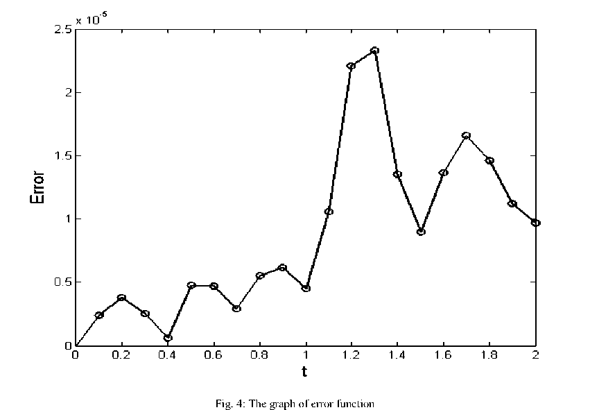
We define the pointwise error for above approximate optimal solution as follows:

E ⁽ t k ) = | ^x * ⁽ t k ) ^- g ^{( x} * ⁽ t k ) ^{- f (} u * ⁽ t k ))|, k = 0,1,..., N .

• V.    Numerical Result

Consider the following non-smooth optimal control problem:

Minimize x ( T )                            (20)

subject to

x ( t ) = - I x ( t ) - 0.5I + u ( t ), t ∈ [0, T ],

x(0)=0.3,0≤x(t)≤1,0≤u(t)≤1,t∈[0,T], where T = 2 . Here, we assume  g(x) = - x - 0.5 ,

µ _n ( x ) = cos( n π x ), x ∈ [0,1] and P = 69, N = 20, M = 10 . We solve the LP problem (15) and obtain the generalized derivative of function g ( x ) = - x - 0.5 as

∂ _xg ( x ) = ∑ a_n ^∗ cos( n π x ), x ∈ [0,1] n = 0

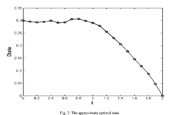
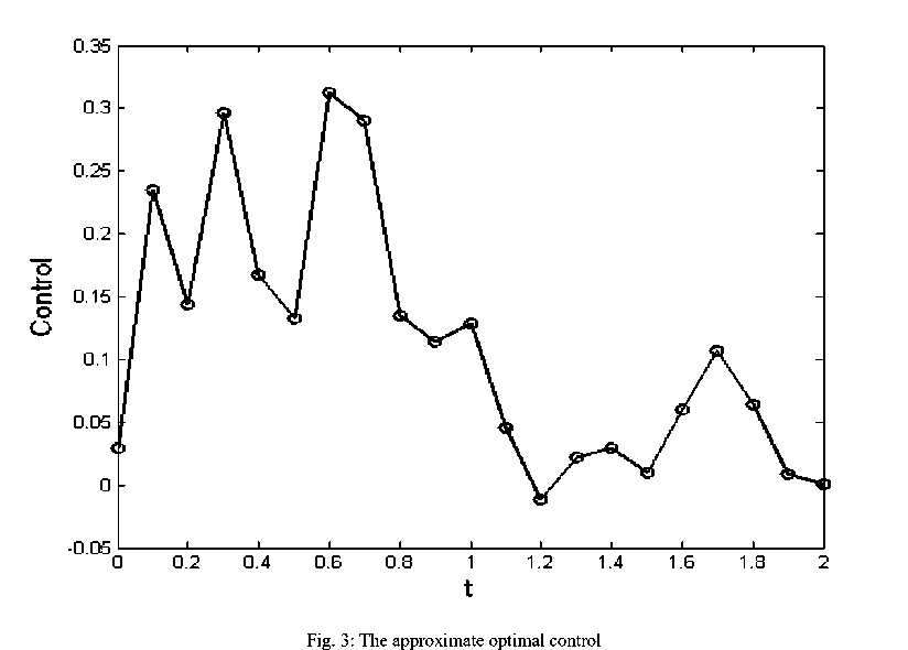
which is shown in Fig. 1. Further, by solving the corresponding smooth NLP (18), we obtain the approximate optimal state and optimal control for the nonsmooth optimal control problem (20) as follows:

x∗(tk)≈xk∗,u∗(tk)≈uk∗,k =0,1,...,20, where they are illustrated in Figs. 2 and 3, respectively. Here the objective function is x (2) = 0 and the error of obtained approximate optimal state and control, corresponding to the relation (19), is shown in Fig. (4). The upper bound for pointwise error is2.33×10-5 .

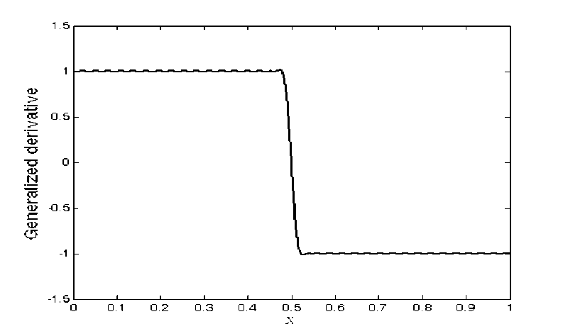
Fig. 1: The graph of generalized derivative

• VI.    Conclusion

In this work, we showed that the non-smooth optimal control problems are converted to the smooth form by using a new practical generalized derivative. Moreover, we showed that the smooth optimal control problems were approximated to the nonlinear programming problem by using the discretization method.

Acknowledgements

The research was supported by a grant from Ferdowsi University of Mashhad (No. MA89187KAM).