Solving a Linear Programming with Fuzzy Constraint and Objective Coefficients

Published Online July 2016 in MECS

In the recent years, the optimal decision making is a difficult matter for managers of the big dynamic companies and organizations. For making optimal decisions the managers are facing different constraints such as the limited financial and human resources. One of the most common and simple tools which is used to achieve the best outcome(such as maximizing the profit or minimization the cost) subject to different constraints is the Linear Programming (LP) methods. In general, a linear programming problem can be written as:

max(min) z = cx subject to

Ax <  b (1) x >  0

In practice, all of the needed information such as с, Л , b are not completely available or determined, or in the other sense, these parameters include uncertainty and they are called fuzzy variables. In the recent years, fuzzy logic and optimization have found many applications in different areas. The fuzzy decision making was introduced by Bellman and Zadeh for the first time in

1970 [1], and the in 1974 the mathematical fuzzy programming was proposed by Tanaka et al [16]. Ramik and Rimanek [14] also dealt with an LP problem with fuzzy parameters in the constraints. Later, Delgado et al. [3] studied a general model for fuzzy LP problems which includes fuzziness both in the coefficients and in the accomplishment of the constraints. The first fuzzy linear programming formulation was discussed by Zimmermann in 1978 [20], and then many other models and methods were suggested by others. Negoita developed a formulation for fuzzy linear programming problem based on the fuzzy coefficient matrix [10]. Then, in 2003 multiobjective fuzzy linear programming problem was established by Zhang et al [18]. In the last years, Erfanian et al. have worked on some concepts of generalized derivative of fuzzy nonsmooth functions, generalized first and second derivative for nonsmooth functions and nonsmooth optimal control[4,5,11,12]

In this paper, linear programming problems with the fuzzy resources and coefficients are discussed. Hence, in section 2, some of the basic definitions and concepts of fuzzy sets and fuzzy optimization are reviewed. In section 3, the concepts of ranking functions are introduced. In section 4, a fuzzy linear programming with fuzzy resources and coefficients is considered, and in section 5, multi-objective fuzzy linear programs are discussed. Finally, in section 6, a practical example is solved and in the last section the results are summarized.

• II.    Preliminaries

In this section, we review some of the definitions and concept of the fuzzy sets and calculus [19].

A.--

Suppose X is an arbitrary universal set. Then a fuzzy subset A in X is defined as follows:

A = { ⁽ x , M A ⁽ x ))| x e X }                ⁽²⁾

where m ( x ): X ^ [ 0,1 ] is the so called membership function.

• B.--

• A fuzzy set A is normal if there exists x0 e X with WA (xo) = 1

C.--

The support of a fuzzy set A is a set which its members have non-zero membership degree, and is defined as follows:

Supp ( A ) = { x e X Ц_А ( x ) >  0 }          (3)

D.--

A weak cut of a fuzzy set is a set which its members belong to the universal set and its membership function in the fuzzy set A has the value equal or greater than a.

H.--

Suppose the triangular fuzzy numbers A and B are ( a , a , a ) and ( b , b , b ) respectively a , b are the centers a , b are the biggest and a , b are the smallest possible values. Then the addition and subtraction of these two numbers are defined as follows:

A © B = ( a , a ₂, a ₃) © ( b , b ₂, b )

= ( a + b , a ₂ + b ₂, a ₃ + b ₃)

A © B = ( a 1 , a ₂, a ₃) © ( b 1 , b ₂, b ₃)

= (a - b ₃, a ₂ - b ₂, a ₃ - b )           (7)

• I .--

• If A and B are the triangular fuzzy numbers in the form of A = (a, b, c), B = (x, y, z), then we have [7]:

A a = [ A ] ^a = { x e X| Ц л ( x ) >  a , a e [0,1] }

In the definition above, if one neglects the equality condition of the membership degree, then the achieved set is called a strong α-cut.

E.--

A fuzzy set A in X = Rⁿ is convex if every a -cut of A for any a (0 <  a <  1) is convex. In other words, a fuzzy set A is convex if and only if for every x , x ₂ e X and X e [ 0,1 ] the following inequality holds:

Ц A ^{[ X} x + ^{(1 - X )} x 2^] >  mini W A ⁽ x ) Ц- A ⁽ x 2^)]

F.--

A fuzzy set A on real numbers R , which satisfies the following condition is called a fuzzy number.

• 1-    A is a convex set.

• 2-    There exist only one unique x e R , such that W A ^{( x} ) = 1.

• 3-    ц ( x ) is piecewise continuous.

G.--

A triangular fuzzy number with the center s the left bound l >  0, and the right bound r >  0 has the following membership function:

x - ( s - 1 )

l

s - l

< x <  s

( ax , by , cz ),

A © B = <  ( az , by , cz ),

( az , by , cx ),

a >  0

a <  0, c >  0

c <  0

W A ⁽ x ) = <

( s + l ) - x

r

0,

s <  x <  s + 1

o . w .

• III.    Ranking of Fuzzy Numbers

In this section, we present a new approach to fuzzy ordinary where for any two triangular fuzzy numbers a = ( s_a , l_a , K a ) and b = ( s b , l b , r ) , a^ b if and only if ^sa <  ^sb , ^sa ^{- l}a <  ^sb ^{- l}b and ^sa ⁺ r a <  ^sb ⁺ r b .

J.--

Assume a = ( s_a , l_a , r ) and b = ( s_b , l_b , r_b ) to be two triangular fuzzy numbers. The definitions of the relations , « , and , ^, are given in below:

a ~ biff ^sa = ^sb , ^s _Q ^- l a = ^sb ^{- l}b , ^sa ⁺ r a = ^sb ⁺ r b , a^bffS a <  ^sb , ^s _a ^- l a <  ^sb ^- l b , $ a + 1 a <  ^sb + r b .   (9)

Remark 1: Denote a ^ b if and only if a ® b or a^b and let 0 = (0,0,0) be a zero triangular fuzzy number. Thus, any a such that a ^ 0, is a zero too.

Lemma 1 : Assume a- Than - a >- -b .

Proof. It is straightforward.

Lemma 2 : Assume a , b , c e F (R). Than,

• 1)    a ^ a for every a (reflexivity);

• 2)   a ^ b ,than b ^ a (symmetry);

• 3)    a ^ b and b ^ c , than a « c (transitivity).

Proof. It is straightforward.

Remark 2: In fact, Lemma up shows that the relation , ^ is an equivalence relation on F (R). Moreover, if a is an element of F ( ), the fuzzy subset of F ()defined by

• [a] = {b e F(R) | a » b}(10)

is called the equivalence fuzzy set of a is thus the set of all elements which are equivalent to a .

Lemma 3: Assume a,b,c e F(R). The relation, < is a partial order onF().

Proof . It is straightforward by evaluation the triple properties: reflexivity, symmetry and transitivity.

Remark 3: We emphasize that the relation ,,is a linear order on F().

Lemma 4 : If a^b and c^d , then a + c^b + d .

Proof. It is straightforward.

• IV. Linear Programming Problem with Fuzzy Resources and Coefficients

Consider the following fuzzy linear programming problem [2, 6, 9, 15]:

n

(c, x) = ^(Xj) = f(x) = max z = L cjxj j=1

subject to     У Дх, <  Bi  (1 < ; <  m )      (11)

j = 1

X j >  0  (1 <  j <  n )

where A , B , c are fuzzy numbers. In this case, we assume that all of fuzzy numbers are triangular. As shown in Figure (1), ever triangular fuzzy number can be cast as 3 real numbers s , l , r , i.e. A = ( s , l , r ).

Now, the model (1) can be written as n max cc, x) = L cxj j=1

s . t .   L ⁽ s j ^{, l}j ^{, r}j ) X j < ^{( t}; , U ; , v i)  ⁽¹ < ^; <  m )

j = 1

x j >  0    (1 <  j <  n )              (12)

Theorem 1 :  For every two fuzzy numbers

A = ( s , l , r ), B = ( s ₂, l ₂, r ₂ )we have A <  B if and only if s _i<  s ₂, S j — l_x <  s ₂ — 1 ₂, s ₁ + r <  s ₂ + r ₂.

Proof. It is straightforward.

Using the above expressions, the model (12) can be converted to a classic linear program as follows:

n max  cc, x) = L cjxj j=1

• s . t .   ILs _u^xj <  t ;

j = 1

LL ^{( s};j - ^lj > ^xj <  t ; - ^u-   ⁽¹ <  ^; <  ^m )

j = 1                                                  (13)

LL ^{( s}j ^{+ r};j ) ^xj <  t ; + v ; j = 1

x j >  0                 (1 <  j <  n )

However, since all numbers involved in constraints are real numbers and all goal coefficients are fuzzy numbers, this problem is an essentially fuzzy LP problem.

K.--

A point x * e X is said to be an optimal solution to the fuzzy LP problem if it holds that (in maximization case) if cc , x > ( c , x ) for all x e X .

L.--

A point x * e X is said to be a no dominated solution to the fuzzy LP problem if there does not exist x * e X such that ( c , x ) >  cc , x * ^ holds.

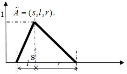
Fig.1. The Fuzzy Number A

V. Multi-Objjective Fuzzy Linear Programming Problems

We consider the following Multi-Objective Linear program (MOLP), which is strongly related to the fuzzy linear programing problem [9,15].

max ( MOLP ) ^

( c ₀ , x , c ₀ , x , c ₀ , x )

s . t .

Dx <  d , x >  0

where l     l   llT c0    (c 01, c02,..., c 0 n ) , c     c  ccT cl = (c11, c12,-.-, C1 n ) , u     u  u     uTn c0    (c 01, c02,..., c0 n ) e д, and the constraint Dx < d is constructed using the model (13).

M.--

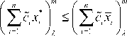
A point x * e X is said to be a complete optimal solution to the (MOLP) problem if it holds that (( c 0 , x * ),(c c , x * ),( c 0 , x * )) T >  (( c 0 , x ),( c c , x ),( c _o ^u , x )) ^T for all x e X .

N.--

A point x * e X is said to be a Pareto optimal solution to the (MOLP) problem if there is no x e X , such that (( c 0 , x * ),( c c , x * ),( c _o ^u , x * )) T <  (( c 0 , x ),( c c , x ),( c _o ^u , x )) T holds.

Theorem 2 : Let point x * e X be a feasible solution to the fuzzy LP problem. c , c ,..., c are determined by the reference functions, i.e., for the triangular fuzzy number c , L and R are respectively the left and right reference functions, and also X level set of c. is represent as interval [ c X , c R ].if

A( c L + (1 - X ) c m ) = L( X + (1 - X ) c 2 m l ) = ...

= L „ ( X c Lo + (1 - X ) c”),

R 1 ( c L + (1 - X ) c m ) = R 2 ( X c L + (1 - X ) c ”) = ...

= R (XcLo + (1 - X) e”), then x* is an optimal solution to the problem if and only if x* is a complete optimal solution to the (MOLP) problem.

Proof. If x ^* is an optimal solution to the fuzzy LP problem, then for any x e X , we have cc , x *^ > ^ c , x ^ . Therefore, for any X e [0,1],

and

That is

So c1m, x*

> ( ^ ^c 0 , ^x ^, ^ ^c 1 , ^x ^, ^ ^c 0 , ^x ^ )  '

Hence x ^* is a complete optimal solution to the (MOLP) problem.

Now if x ^* is a complete optimal solution to the (MOLP) problem, then for all x e X , we have

(( c L , x'

, c 1 ^m , x ^*

T

T

i.e., n   nnn

2 cL x >2 cL x,, 2 cm x* >2 cm x, i=1                i=1            i=1

and nn Er *

ci 0 xi >2 ci 0 xi. i=1

Then nn

2(XcL + (1 -X)cm-)x* > 2(XcL + (1 -X)cm)x,, VX e[0,1]. i=1

According to Eq. (15), we have

3 X 1 e [0,1], X c L + (1 - X ) c m = c X , i = 1,2,..., n.

(if X = 1, it is clear that c L = c m .)

So fcLx* > VcLx. ZX1 IZX i=1

Similarly, nn

2(XcR + (1 -X)cm)x* > 2(Xc,^0 + (1 -X)cm)x, VX e [0,1]. i=1

According to Eq. (16), we have

3 X 2 e [0,1], X c R + (1 - X ) c m = c R x , i = 1,2,..., n .

(if X = 1, it is clear that c^R = c m .)

So

2 c z X x , .

i = 1

For fuzzy numbers ( c )_L ^ , i = 1,2,..., n, since the reference functions L _z and R_t are strictly decreasing, so X and X can take every value in the interval [0,1] .We can take the proper X to \ = X = X as well as suggested also in [6]. Then, we have

and nn

ZciR x -ZcXxi,  VXg[0,1], i=1                i=1

Zmx* -zZcmx  for X = 1, i=1 i             i=1 i for any Xg [0,1]. Therefore, x* is an optimal solution to the fuzzy LP problem and the proof is completed.

Remark 4 : For the fuzzy LP problem, if the fuzzy coefficients c , i = 1,2,..., n, have the same shapes, the eqations (15) and (16) hold.

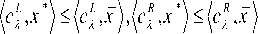
Theorem 3 : Let point x * g X be a feasible solution to the fuzzy LP problem. Then x ^* is a no dominated solution to the problem if and only if x ^* is a Pareto optimal solution to the (MOLP) problem.

Proof. Let x * g X be a no dominated solution to the fuzzy LP problem. On the contrary, we suppose that there exists an x g X such that

(ccR,x*Ycm,x*YcRR,x*)) -((cL,x),(cm,x),(cR,x)) , i.e., n   nnn

Z cL x* -Z cL x, Z cm x* -Z cm xi i=1                 i=1             i=1

and nn

Er *

c i 0 x i ^- Z c i 0 x i .

i=1

Then nn

Z(XL + (1 - X)cm)x, - Z(XcL + (1 - X)cm)x- , VX g [0,1]. i =1

According to Eq.(15), we have x. G[0,1],XcjLL + (1 -X)cm = cL1,i = 1,2,...,n.

(if X = 1, it is clear that c L = c m .)

So nn

У c L x * - У c L xi .

1X1 i1

i=1

Similarly, nn

Z ( X R + (1 - X ) c m ) x * - Z ( c^  + (1 - X ) c m ) x i , V X g [0,1].

i =1

According to Eq. (16), we have

3 ^ 2 g [0,1], X c R + (1 - X ) c m = c X , i = 1,2,..., n .

(if X = 1, it is clear that c^R = c m .)

So nn Er *

ciX xi - Z ciX xi. i=1

And for X1 = X2 = 1, we have nn

Zcmx* -Zcmx. i=1

That is c , x     c , x ^* .

However, this contradicts the assumption that x * g X is a no dominated solution to the fuzzy LP problem.

On the other side, let x * g X be a Pareto optimal solution to the (MOLP) problem.

If x* is not a no dominated solution to the problem, then there exists x g X such that^c,x^tc,x*Y Therefore, = for any X g [0,1], we have

and

That is

and m c

) <  Rd, , x^ .

Hence, for Я = 0 and X = 1, we have

Cc L , x ) > ( c L , x *), R m™ , x^ >  Rm™ , x *Y C r R , x ) > ( c^R , x *) .

It contradicts the assumption that x * e X is a Pareto optimal solution to the (MOLP) problem.

Consider a multiple objective optimization problem with k fuzzy goals z , z ,..., z , which are introduced by fuzzy sets Z , i = 1,2,..., k , and fuzzy constraints are d , d ,..., d   , which are shown by fuzzy sets

D, j = 1,..., m . By generalizing the analogy from the single objective function, the resulting fuzzy decision is given as

Z 1    Z 2    ...   Z k D 1 D 2    ...   D m .

In terms of corresponding membership values for the fuzzy goals and the fuzzy constraints, the resulting decision is

^Д ( X ) = ппп[ д ., ^d^ ^].

An optimum solution X ^* is one at which the membership function of the resulting decision f is maximum. That is

A f ⁽ X * ) = ^max A f ⁽ X ^).

The shape of the membership functions such as a linear, concave, or convex function, for various objectives and constraints, can affect the optimum solution significantly. A linear approximation has been most commonly used because of simplicity and expediency [17].

Applying the triangular fuzzy parameters as triangular fuzzy number the MOLP will be written as follows:

max2, =£(cc,c1,c")ijxj j =1

S t.      'Lsijxj < ti j =1

j^(sij - 1ij)xj

У⁽Sij + rij)x,< ti + v,   ⁽¹< i< m)

j =1

x« > 0.                  (1 < j< n)

Since we get z as (z1,z2,z3) where, z,1 = £(cc)ijxj >        i = 1>2—>k j =1

zi2 = £ c -c‘) ijxj> i = I2’-’k j =1

zi3 = £(cc + c“)ijxj,  i = 1,2,...,k.

j =1

Thus the objective function of the problem (17) becomes

123  123

max(z₁ ,z₂ ,z₃ ,...,z_k ,z_k ,z_k)

To solve this multi-objective problem we use Pareto’s method to form weighted objective function

123  3

max wxzx + wz + w^zx +... + w3kzk, and with the same constraints as in (17) along with the additional constraint Уw k = S. [13]

• VI.    Numerical Example

In this section, we present a simple example to illustrate the above concepts.

Example. A Company would like to produce two products A, B . There are 150 man-hour and 120 kg material available. In addition, suppose the gained profit from producing each unit of A andB is almost known. The aim of the company is to maximize the overall profit of producing these two products.

Suppose x is the production amount for the product A , andx is the production amount for the product B .

So, this problem can be modeled as:

max z = f (xpx₂) = c_xx_x + c₂x₂

s.t.

(5,2,1)x₁ + (4,3,1)x ₂< (150,50,40)

(3,2,1)x_x + (4,2,1)x₂< (120,40,30) xpx₂ > 0

The membership function is:

Ac, ^(x) = *

x - 40

5,

60 - x

15   ,

0,

40 < x< 45

45 < x< 60

o.w.

n maxz. = У(сс, c1, cu).x. i = 1,2,..., k, i                                          ij j j =1

	' x - 30	30 < x < 36
	6,
ц=г(x) ='	40 - x	36 < x < 40
	4,
	0,	o.w.

Therefore, the objective function will be as follows:

max z = f (x₁, x₂) = (40,45,60) x_x + (30,36,40) x₂

According to the discussed algorithm, the human resources constraint can be written as:

5x + 4x₂< 150

< 3x +1 x₂< 100

6x + 5x₂< 190

Also, the constraint for the available materials can be cast as:

^3x + 4x₂< 120

< 1 x + 2x₂< 80

4x + 5x₂< 150

Now, we can rewrite the above problem as a linear programming:

max z = 40x + 30x₂

+ 45x + 36x₂

+ 60x + 40x₂

s.t.

5x₁ + 4x₂< 150

3x, +1 x₂< 100

6x. + 5x₂< 190

3x. + 4x₂< 120

1 xj + 2x₂< 80

4x, + 5x₂< 150

x_x > 0

x₂ > 0

After solving the above problem using LINGO, the following optimal Pareto solution is achieved:

(x*, x*) = (30,0)

Therefore, the above solution is a non-dominated. Here, for solving the linear programming, we maximize the objective-weighted form of the problem as follows:

max z (x, x₂) = w_x (40x_x + 3 0x₂)

+ w₂ (45x + 36x₂)

+ w₃ (60x + 40x₂)

The optimal solution of the above problem can be found using different weights. Note that ^ w. = 1.

i=1

Table 1. The Optimal Solution of Example

Optimal Solution	w1	w2	w3
(30,0)	0	0.5	0.5
(30,0)	0.5	0	0.5
(30,0)	0.5	0.5	0

The optimal solution will be presented as:

(x*, x*) = (30,0)

Therefore, max z = f (x*, x*) = f (30,0) = 30q + 0c2

^ (x) = ’	x -1200
	150 1800 - x
	450 0,

1200 < x < 1350

1350 < x < 1800

o.w.

• VII.    Conclusion

In this paper, the linear programming problems with fuzzy budget and constraints have been discussed. An algorithm to solve such problems has been discussed and for more illustration the mentioned algorithm has been applied to a numerical example. As a result of this example, it has been highlighted that the solution is independent from the chosen weights.