Solving Economic Load Dispatch Problem Using Particle Swarm Optimization Technique

Published Online November 2012 in MECS

The economic load dispatch (ELD) of power generating units has always occupied an important position in the electric power industry. ELD is a computational process where the total required generation is distributed among the generation units in operation, by minimizing the selected cost criterion, subject to load and operational constraints. For any specified load condition, ELD determines the power output of each plant (and each generating unit within the plant) which will minimize the overall cost of fuel needed to serve the system load [1]. ELD is used in real-time energy management power system control by most programs to allocate the total generation among the available units. ELD focuses upon coordinating the production cost at all power plants operating on the system.

In the traditional ELD problem, the cost function for each generator has been approximately represented by a single quadratic function and is solved using mathematical programming based optimization techniques such as lambda iteration method, gradientbased method, etc [2]. These methods require incremental fuel cost curves which are piecewise linear and monotonically increasing to find the global optimal solution.

Dynamic programming (DP) method [3] is one of the approaches to solve the non-linear and discontinuous ELD problem, but it suffers from the problem of “curse of dimensionality” or local optimality. In order to overcome this problem, several alternative methods have been developed such as genetic algorithm [4], evolutionary programming [5, 6], tabu search [7], neural network [8], and particle swarm optimization [911].

Particle swarm optimization (PSO) is suggested by Kennedy and Eberhart based on the analogy of swarm of birds and school of fish [12]. PSO mimics the behavior of individuals in a swarm to maximize the survival of the species. In PSO, each individual makes his decision using his own experience together with other individuals’ experiences. The algorithm, which is based on a metaphor of social interaction, searches a space by adjusting the trajectories of moving points in a multidimensional space. The individual particles are drawn stochastically toward the position of present velocity of each individual, their own previous best performance, and the best previous performance of their neighbors. The main advantages of the PSO algorithm are summarized as: simple concept, easy implementation, robustness to control parameters, and computational efficiency when compared with mathematical algorithms and other heuristic optimization techniques [12, 13]. PSO can be easily applied to nonlinear and non-continuous optimization problem.

In this paper, a PSO technique for solving the ELD problem in power system is proposed. The feasibility of the proposed method was demonstrated for a three units and six units system and the results were compared with quadratic programming method [14]. The results indicate the applicability of the proposed method to the practical ELD problem.

The rest of this paper is organized as follow. Section 2 presents the ELD formulation. Section 3 presents quadratic programming method. Section 4 proposes PSO technique to solve ELD problem. Results and discussions are given in section 5, and section 6 gives some conclusions.

• II.    Economic Load Dispatch Formulation

The objective of an ELD problem is to find the optimal combination of power generations that minimizes the total generation cost while satisfying an equality constraint and inequality constraints. The fuel cost curve for any unit is assumed to be approximated by segments of quadratic functions of the active power output of the generator. For a given power system network, the problem may be described as optimization (minimization) of total fuel cost as defined by (1) under a set of operating constraints.

nn

F t = Z F ( P i ) = № P 2 + b i P i + C i )     (1)

i = 1                    i = 1

where F is total fuel cost of generation in the system ($/hr), a i , b i , and c i are the cost coefficient of the i th generator, P i is the power generated by the i th unit and n is the number of generators.

The cost is minimized subjected to the following generator capacities and active power balance constraints.

P i < P i ^ P i,max for i = 1,2, - , П         (2)

where P i, min and P i, max are the minimum and maximum power output of the i th unit.

n

P d = Z P - P loss                       (3)

i = 1

where P D is the total power demand and P Loss is total transmission loss.

The transmission loss PLoss can be calculated by using B matrix technique and is defined by (4) as, nn

P Loss = ZZ P i B-P                   (4)

i = 1 j = 1

where B_i j ‘s are the elements of loss coefficient matrix B .

• III.    Quadratic Programming Method

A linearly constrained optimization problem with a quadratic objective function is called a Quadratic Program (QP). Due to its numerous applications; quadratic programming is often viewed as a discipline in and of itself. Quadratic programming is an efficient optimization technique to trace the global minimum if the objective function is quadratic and the constraints are linear. Quadratic programming is used recursively from the lowest incremental cost regions to highest incremental cost region to find the optimum allocation. Once the limits are obtained and the data are rearranged in such a manner that the incremental cost limits of all the plants are in ascending order.

The general quadratic programming can be written as:

1 T

Minimize f ( x ) = cx + — x Qx            (5)

Subject to Ax <  b and x >  0               (6)

where c is an n -dimensional row vector describing the coefficients of the linear terms in the objective function, and Q is an ( n × n ) symmetric matrix describing the coefficients of the quadratic terms. If a constant term exists it is dropped from the model. As in linear programming, the decision variables are denoted by the n -dimensional column vector x , and the constraints are defined by an ( m × n ) A matrix and an m -dimensional column vector b of right-hand-side coefficients. We assume that a feasible solution exists and that the constraint region is bounded. When the objective function f ( x ) is strictly convex for all feasible points the problem has a unique local minimum which is also the global minimum. A sufficient condition to guarantee strictly convexity is for Q to be positive definite.

If there are only equality constraints, then the QP can be solved by a linear system. Otherwise, a variety of methods for solving the QP are commonly used, namely; interior point, active set, conjugate gradient, extensions of the simplex algorithm etc. The direction search algorithm is minor variation of quadratic programming for discontinuous search space. For every demand the following search mechanism is followed between lower and upper limits of those particular plants. For meeting any demand the algorithm is explained in the following steps:

• 1)    Assume all the plants are operating at lowest incremental cost limits.

• 2)    Substitute P = L_t + (U_t — L_t ) X_t ,

where 0 <  X_t <  1 and make the objective function quadratic and make the constraints linear by omitting the higher order terms.

• 3)    Solve the ELD using quadratic programming recursively to find the allocation and incremental cost for each plant within limits of that plant.

• 4)    If there is no limit violation for any plant for that particular piece, then it is a local solution.

• 5)    If for any allocation for a plant, it is violating the limit, it should be fixed to that limit and the remaining plants only should be considered for next iteration.

• 6)    Repeat steps 2, 3, and 4 till a solution is

achieved within a specified tolerance.

• IV.    Overview of Particle Swarm Optimization

Natural creatures sometime behave as a Swarm. One of the main streams of artificial life researches is to examine how natural creatures behave as a Swarm and reconfigure the Swarm models inside the computer. Kennedy and Eberhart develop PSO based on analogy of the swarm of birds and fish school. Each individual exchanges previous experiences among themselves [12]. PSO as an optimization tool provides a population based search procedure in which individuals called particles change their position with time. In a PSO system, particles fly around in a multi dimensional search space. During flight each particles adjust its position according its own experience and the experience of the neighboring particles, making use of the best position encountered by itself and its neighbors.

N      Dimension of the optimization problem

(number of decision variables)

N      Number of particles in the swarm r ,r    Two separately generated uniformly distributed random numbers in the range [0, 1]

In the multi-dimensional space where the optimal solution is sought, each particle in the swarm is moved toward the optimal point by adding a velocity with its position. The velocity of a particle is influenced by three components, namely, inertial, cognitive, and social. The inertial component simulates the inertial behavior of the bird to fly in the previous direction. The cognitive component models the memory of the bird about its previous best position, and the social component models the memory of the bird about the best position among the particles. The particles move around the multi-dimensional search space until they find the optimal solution. The modified velocity of each agent can be calculated using the current velocity and the distance from Pbest and Gbest as given below.

V j = w x V j - 1 + C 1 X Г 1 x ( pbes j - X t ^{- 1} ) + C x r x ( Gbest t ^{- 1} - X t ^{- 1} )

i = 1,2,-,Nd ; j = 1,2,-,Npar     ^

The following weighting function is usually utilized:

to = to

where,

max

to , to max , min

Iter„ max

Iter

((co —co ■ max     min

Iter max

\

x Iter

Initial and final weights

Maximum iteration number

Current iteration number

Using the above equation, a certain velocity, which gradually gets close to Pbest and Gbest, can be calculated. The current position (searching point in the solution space), each individual moves from the current position to the next one by the modified velocity in (7) using the following equation:

x t = xt.-1 + vl.

ij          ij          ij                                                      (8)

where, t         Iteration count

V t      Dimension i of the velocity of particle j at iteration t

X t      Dimension i of the position of particle j at iteration t w       Inertia weight

C , C Acceleration coefficients

Pbest ^t Dimension i of the own best position of particle j until iteration t

Gbest^t Dimension i of the best particle in the swarm at iteration t

Suitable selection of inertia weight in above equation provides a balance between global and local explorations, thus requiring less number of iterations on an average to find a sufficient optimal solution. As originally developed, inertia weight often decreases linearly from about 0.9 to 0.4 during a run.

The algorithmic steps involved in particle swarm optimization technique are as follows:

• 1)    Select the various parameters of PSO.

• 2)    Initialize a population of particles with random positions and velocities in the problem space.

• 3)    Evaluate the desired optimization fitness function for each particle.

• 4)    For each individual particle, compare the particles fitness value with its Pbest. If the current value is better than the Pbest value, then set this value as the Pbest for agent i.

• 5)    Identify the particle that has the best fitness value. The value of its fitness function is identified as Gbest.

• 6)    Compute the new velocities and positions of the particles according to equation (7) & (8).

• 7)    Repeat steps 3-6 until the stopping criterion of maximum generations is met.

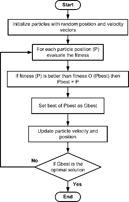
The procedure of the particle swarm optimization technique can be summarized in the flowchart of Fig. 1.

Case Study-1: 3-units system

In this case, a simple power system consists of three-unit thermal power plant is used to demonstrate how the work of the proposed approach. Characteristics of thermal units are given in Table 1, the following coefficient matrix B ij losses.

Table 1: Generating unit capacity and coefficients

Unit	min (MW)	max (MW)	a i ($/MW2)	b i ($/MW)	c i ($)
1	50	250	0.00525	8.663	328.13
2	5	150	0.00609	10.04	136.91
3	15	100	0.00592	9.76	59.16

в ij

0.000136 0.0000175 0.0001840.000175 0.0001540 0.0002830.000184 0.0002830 0.001610

Fig. 1: The flowchart of PSO technique

By using the proposed PSO technique obtained the results as shown in Table 2 and Table 3. Test results in Table 2 for 3-generator system with load change from 250 MW to 400 MW without taking into account transmission losses. Table 3 shows the optimal power output, total cost of generation, as well as active power loss for the power demands of 275 MW, 300 MW and 350 MW. Table 3 shows that the PSO method is better than conventional method (quadratic programming) for each loading.

• V.    Results And Discussions

To verify the feasibility and effectiveness of the proposed PSO algorithm, two different power systems were tested one is three generating units [15] and other is six generating units [16, 17]. Results of proposed particle swarm optimization (PSO) are compared with quadratic programming methods. A reasonable B-loss coefficients matrix of power system network has been employed to calculate the transmission loss. The software has been written in the MATLAB-7 language.

Table 2: Best power output for 3-generator system (without loss)

P demand (MW)	P1 (MW)	P2 (MW)	P3 (MW)	Fcost ($/hr)
250	151.09	42.04	56.87	2959.98
275	173.00	37.78	64.22	3219.23
300	186.18	52.70	61.12	3483.73
325	195.85	60.96	68.19	3749.95
350	205.57	61.51	82.92	4017.52
375	219.67	68.15	87.18	4288.92
400	210.38	89.70	99.92	4563.00

Table 3: Best power output for 3-generator system

P demand (MW)	Method	P1 (MW)	P2 (MW)	P3 (MW)	PLoss (MW)	Fcost ($/hr)
275	Conv.	193.82	74.78	15.00	8.61	3333.14
	PSO	189.31	79.13	15.00	8.44	3332.69
300	Conv.	207.68	87.40	15.00	10.08	3621.53
	PSO	212.56	82.48	15.00	10.04	3620.09
350	Conv.	235.58	112.89	15.00	13.47	4215.18
	PSO	228.15	119.73	15.00	12.88	4211.08

Case Study-2: 6-units system

In this case, a standard six-unit thermal power plant (IEEE 30 bus test system) is used to demonstrate how the work of the proposed approach, as shown in Fig. 2. Characteristics of thermal units are given in Table 4, the following coefficient matrix Bij losses.

The simulation results with the proposed PSO technique respectively are shown in Table 5, Table 6 and Table 7 with the variation of loading 600 MW, 700 MW and 800 MW. From the simulation results show that the generation output of each unit is obtained correction reduces the total cost of generation and transmission losses when compared with the conventional method (quadratic programming method).

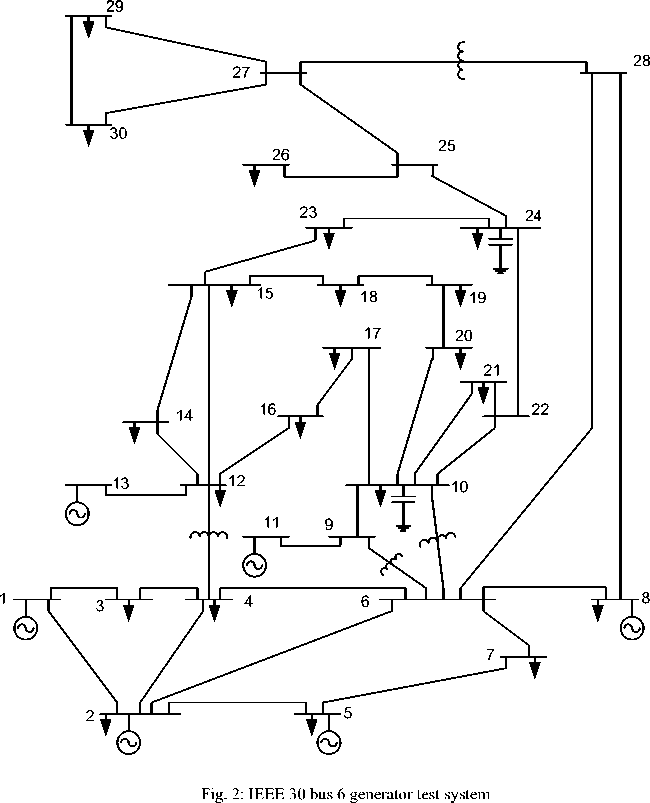
Table 4: Generating unit capacity and coefficients

Unit	P min (MW)	P max (MW)	a i ($/MW2)	b i ($/MW)	c i ($)
1	10	125	0.15240	38.53973	756.79886
2	10	150	0.10587	46.15916	451.32513
3	35	225	0.02803	40.39655	1049.9977
4	35	210	0.03546	38.30553	1243.5311
5	130	325	0.02111	36.32782	1658.5596
6	125	315	0.01799	38.27041	1356.6592

Table 5: Best power output for 6-generator system (P D = 600 MW)

Unit Output	Conventional	PSO
P1 (MW)	23.90	23.84
P2 (MW)	10.00	10.00
P3 (MW)	95.63	95.57
P4 (MW)	100.70	100.52
P5 (MW)	202.82	202.78
P6 (MW)	182.02	181.52
Total power output (MW)	615.07	614.23
Total generation cost ($/hr)	32096.58	32094.69
Power losses (MW)	15.07	14.23

Table 6: Best power output for 6-generator system (PD = 700 MW)

Unit Output	Conventional	PSO
P1 (MW)	28.33	28.28
P2 (MW)	10.00	10.00
P3 (MW)	118.95	119.02
P4 (MW)	118.67	118.79
P5 (MW)	230.75	230.78
P6 (MW)	212.80	212.56
Total power output (MW)	719.50	719.43
Total generation cost ($/hr)	36914.01	36912.16
Power losses (MW)	19.50	19.43

Table 7: Best power output for 6-generator system (P D = 800 MW)

Unit Output	Conventional	PSO
P1 (MW)	32.63	32.67
P2 (MW)	14.48	14.45
P3 (MW)	141.54	141.73
P4 (MW)	136.04	136.56
P5 (MW)	257.65	257.37
P6 (MW)	243.00	242.54
Total power output (MW)	825.34	825.32
Total generation cost ($/hr)	41898.45	41896.66
Power losses (MW)	25.34	25.32

B

0.000140

0.000017

0.000015

0.000019

0.000026

0.000022

0 . 000017

0 . 000060

0 . 000013

0 . 000016

0 . 000015

0 . 000020

0.000015

0.000013

0.000065

0.000017

0.000024

0.000019

0.000019

0.000016

0.000017

0.000071

0.000030

0.000025

0.000026

0.000015

0.000024

0.000030

0.000069

0.000032

0.000022

0.000020

0.000019

0.000025

0.000032

0.000085

• VI.    Conclusion

This paper presents an efficient and simple approach for solving the economic load dispatch (ELD) problem. This paper demonstrates with clarity, chronological development and successful application of PSO technique to the solution of ELD. Two test systems 3-generator and 6-generator systems have been tested and the results are compared with quadratic programming method. The proposed approach is relatively simple, reliable and efficient and suitable for practical applications.