Some notes on linear programming problems

Бюллетень науки и практики / Bulletin of Science and Practice

UDC 519.852.2                                     

Nowadays, the ability to apply theoretical knowledge in solving practical problems is becoming a decisive factor for the study of any discipline. In particular, based on many years of experience in teaching business mathematics at an economic university, the authors consider it necessary to demonstrate the solution of some economic problems with the help of mathematical apparatus [1, 2].

If we fail to improve mathematics education in a way that takes into account the needs of today's world and students, we are in danger of turning mathematics into an increasingly "dead language" and alienating groups of students whose mathematical potential remains undeveloped [3, 4].

In many cases of investment production projects, deposits are returned in the same payment stream or other type of payment. It is called an "annuity" [5].

The subject of mathematical programming is the study of mathematical methods, the study and solution of extreme problems. Mathematical programming methods are used to find the extremum of multidimensional functions with given multidimensional constraints. The function for

(ос) CD which the extreme value is searched is called the objective function of the problem. Constraints on unknown variables are written as a system of equations or inequalities.

A lot of fundamental works are devoted to the methods of linear programming. Mathematician J. Danzig introduced the concept of linear programming and in 1949 proposed an algorithm called the simplex method [8].

Let’s consider constructing mathematical models of some simple economic problems.

The raw material use problem. In the production of n types of products, m types of raw materials are used. Let's denote by S (i = 1, m) types of raw materials; bi — stocks of raw materials of type i; Pj, j = 1, n — types of products; aij — number of units of raw materials of type i , for the production of a unit of product j ; Cj— the amount of profit received from the sale of the unit of product j . Let хj — number of units of product j , that needs to be produced. Then the mathematical model of the problem can be represented as follows.

Find the maximum value of a linear function

L = Cx + Cx +...+Cx

11   22      nn subject to constraints ax + a12x2 +... + alnxn < b ax + a22x2 +... + a2nxn < b2

a m 1 x 1 ⁺ a m 2 x 2 ⁺ ... ⁺ a mn x n <  ^bm

X j >  0 ( j = 1, n )

The diet problem. Let the diet contain m types of nutrients in an amount of at least b (i = 1, m) units, and it is necessary to use n types of feed. To compile a mathematical model of the problem, let's denote by ay (i = 1, m; j = 1, n) — number of units of nutrient i, contained in the unit of feed j ; C — per unit cost of feed j ; xj— number of units of feed j in the daily diet.

It is necessary to find the minimum value of a linear function

L = Cx + C2x2 + ...+Cnxn

subject to constraints ax + al2x2 +... + alnxn > b a21xt + a22x2 +... + a2nxn > b2

a  x. + a  x.. +... + ax„ > h m1 1     m 2 2          mn n     m

X j >  0 ( j = 1, n )

Definition . Linear programming is a field of mathematical programming, which is a branch of mathematics and studies methods for solving the extreme values of a linear function of a finite number of variables, on the unknowns of which linear constraints are imposed.

This linear function is called the objective function, and constraints, which are quantitative relationships between variables that express the conditions and requirements of an economic problem, and are mathematically written as equations or inequalities, are called a system of constraints.

Definition . A set of relations consisting of a linear objective function and linear constraints on its variables is called a mathematical model of linear programming.

A linear function L = C 1 X 1 + C 2 x 2 + ... + C n x n ^ min is given and a system of linear constraints:

anxx + al2x2 +... + alnxn < b

a x, + a^x0 +... + a-,„x„ < b

21 1    22 2         2 nn     2

a x, + a  x2 +... + amx < bm m1 1     m2 2   ...     mn n     m

xj - 0 (j = 1, n)

where a _ij , b _i and C _j — are specified constant values.

Find such non-negative values of x1, x2,...,xn , that satisfy the constraint system (1) and give a minimum value to the linear function.

As noted earlier, in a constraints’ system (1), all b (i = 1, m) can be considered as non- negative. The constraints’ system (1) can be either linear or nonlinear.

All or some of the equations of a system of constraints can be written as inequalities.

If all constraints (1) are given by equations and variables x _j are non-negative, this type of model is called canonical. If at least one constraint is an inequality, then the model is non-canonical.

Basic Definitions. Solution of the system of n linear equations are called such values ( a 1 , a ₂,..., a _n ) , which after substitution x 1 = a 1 , x₂ = a ₂ ,..., x n = a n into each equation of the system, turn it into correct numerical equation.

Definition. A basis solution is a solution in which all free variables are equal to zero.

Definition . A feasible solution is a basic non-negative solution.

Definition . The feasible solution of the LP problem given in the standard form is an ordered set of numbers ( x 1 , x 2 ,..., x_n ) , satisfying the constraints, this is the point in the n — dimensional space. The set of feasible solutions forms the domain of feasible solutions to the LP problem.

Definition . A feasible solution in which the objective function reaches its extreme value is called the optimal solution and is denoted by x опт .

Definition . A reference solution is said to be non-degenerate if the number of its nonzero coordinates is equal to the rank of the system, otherwise it is degenerate.

Theorem (on the replacement of linear inequality by a linear equation). Every solution x = (a, a2,...,an) of inequality a1 x1 + a2x2 +... + anxn

Thus, if the constraint system contains inequalities (in which case the linear programming problem is said to be given in a standard form), then by introducing an additional variable into each inequality, the system can be transformed into a system of equations. Additional variables are called balance or slack variables.

This leads to the rule of transition from the non-canonical form of the linear programming problem to the canonical one. To get to the canonical form of the problem, you need to introduce a balance variable into each inequality. At the sign of inequality <  the balance variable is introduced into the inequality with a plus sign, with an inequality sign >  with a minus sign. Balance variables are not introduced into the objective function.

Example. Translate inequalities into equations:

• a)    ax + a₂x₂ + ... + a_nx_n ^ b

  .

  
  

  .

  
  

• b)    ax + a₂x₂ + ... + a_nx_n >  b

Solution .

• а) ax + a₂x₂ + ... + a_nx_n ^ b ^ ax + a₂x₂ + - + a_nx_n + x_n+ j = b, x_n+ j >  0.

• b) a 1 x 1 + a 2 x 2 + ... + a n x n >  b ^ a 1 x 1 + a 2 x 2 + ... + a n x n - x_{n + 1} = b , x_{n + 1} >  0.

Theorem (On the extremum of an objective function in a bounded domain). If the domain of feasible solutions given by the constraint system of the LP problem is closed and bounded, then the optimal solution of the LP problem exists, and at least one of the supporting solutions of the constraint system is the optimal solution of this problem.

Theorem. (On the extremum of an objective function in an unbounded domain). If the domain of feasible solutions is unbounded, then the optimal solution exists and coincides with at least one of the support solutions if and only if the objective function is bounded from above for maximum problems or from below for minimum problems.

If the conditions of the theorem do not hold, then the objective function is said to be unconstrained in the domain of feasible solutions.

The graphical method is based on the geometric interpretation of the LP problem and is used mainly in solving problems of two-dimensional space.

Consider the problem of linear programming, the system of constraints of which is given in the form of inequalities. Find the maximum value of a linear function

L x = c.x . + cx., + ... + cx 11  22       nn

subject to constraints

a x, + a x₂ + ... + a, x <  b, 11 1     12 2           1 nn     1

a 21 x 1 ⁺ a 22 x 2 ⁺ ... ⁺ a 2 n^xn <  ^b 2

a x + a x + ... + a x < b m 1 1      m 2 2           mn n     m

^xj >  0 ( j = 1, n )

Set of numbers x ₁ , x ₂ , ..., x_n , satisfying constraints (2) and (3) is called a solution. If the system of inequalities (2) under condition (3) has at least one solution, it is called compatible, otherwise it is called incompatible. A linear programming problem in the standard form with two variables is

L ( x ) = cx + c₂x₂ ^ max a_xxx_x + a₁₂x₂ <  b a₂x + a₂₂x₂ <  b

ax + a.x <  b, m 1 1      m 2 2      m

x . > 0 ( j = 1,2 )

Each inequality of this system geometrically defines a semi-plane with a boundary line a ^ + atXi = b ( i = 1, m ) . This means that the line divides the plane into two semi-planes, one of which is true for our inequality, and the other of which is the opposite.

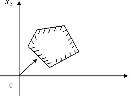
Conditions for non-negativity of variables x >  0, x ₂ >  0 cause this region to be in the first coordinate quadrant.

To find the extreme value of the objective function in the graphical solution of linear programming problems, is used the vector gradL on the plane x1Ox2, which we denote by N . This vector shows the direction of the fastest change of the objective function, it is equal to aL-, d gradL = N = — 61 + dx

where e ₁ and e ₂

— unit vectors on axes ox and Ox ₂ respectively. Thus, N = —, ^d L

V ^s x 1   a x ₂

.

Coordinates of the vector N are the coefficients of the objective function L ( x ) .

Algorithm for solving linear programming problems by graphical method.

• 1.    Finding the feasible region from the problem constraint system.

• 2.    Building a vector N .

• 3.    Drawing the level line L ₀ , perpendicular to N .

• 4.    Move the level line in the direction of the vector N for maximization problems and in the opposite direction to N for minimization tasks. This movement is carried out until the level line has only one point in common with the feasible region of solutions. This point will be the extremum point of the objective function in the feasible region of solutions, i.e. it will be the optimal solution of the LP problem.

• 5.    Find the coordinates of the extremum point and the value of the objective function in it.

If it turns out that the level line is parallel to one of the sides of the feasible region of solutions, then the LP problem will have an infinite number of solutions.

If the feasible region of solutions is an unbounded area, then the objective function can be unlimited.

The LP problem may be unsolvable when the constraints that define its feasible region of solutions are conflicting.

Example . Solve the linear programming problem

L ( x ) = — 6 — X j + 4 x₂ ^ max

'^X 1 - x ₂ >- 2,       (1)

< X 1 + x 2 <  4,         (2)

^ x >  0,(3) x ₂ >  0 (4)

Solution. Let's construct a feasible region of solutions (Figure. Numerate the task constraints. In a rectangular Cartesian coordinate system, we construct a straight line x_x — x₂ = — 2 , conforming to the constraint (1). Let us find which of the two semi-planes is the domain of inequality solutions. For example, the line (1) does not pass through the origin, so we substitute the coordinates of the point O(0, 0) in the first constraint 0 — 0 > — 2 . We get the correct strict inequality of 0 > -2. Hence, point O lies in the semi-plane of the solutions. In the same way, we draw straight lines (2)–(4).

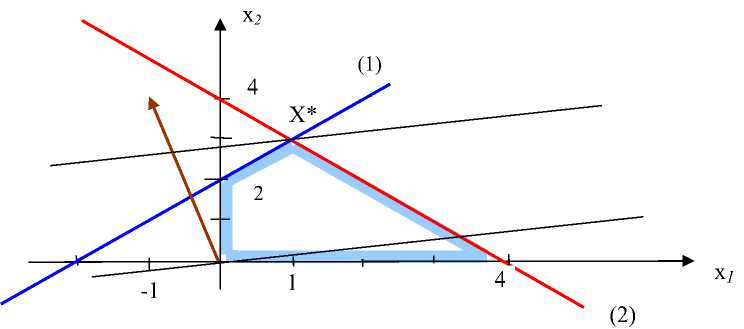
We found grad L = — i + 4 j , draw a level line of the function, perpendicular to the gradient, move it parallel to itself in the direction grad L . This line passes through the point X* of the intersection of the lines that limit the feasible region of solutions and correspond to inequalities (1) and (2).

Determine the coordinates of the point X* by solving the system:

Г X j — x₂ [ X j + x₂

= — 2

= 4.

Get Х*(1, 3). Calculate L ( Х *) = — 6 — 1 + 4 • 3 = 5 .

So, max L (1; 3) = 5.