Spatial Temporal Dynamics and Risk Zonation of Dengue Fever, Dengue Hemorrhagic Fever, and Dengue Shock Syndrome in Thailand

Dengue fever (DF), and its more severe forms, dengue hemorrhagic fever (DHF) and dengue shock syndrome (DSS), is the most important arthropod-transmitted viral disease affecting humans in the world today [1]. The objective of this study was to analyze the epidemic outbreak patterns of DF/DHF/DSS in Chachoengsao province, central part of Thailand, in terms of geospatial distribution and risk area identification. The methodology and the results could be useful for public health officers to develop a system to monitor and prevent DF/DHF/DSS outbreaks.

Vector borne diseases are the most common worldwide health hazard and represent a constant and serious risk to a large part of the world’s population [2]. Among these diseases, dengue fever, especially known in Southern Asia, is sweeping the world, hitting countries with tropical and warm climates. It is transmitted to humans by the mosquito of the genus Aedes and exists in two forms: the Dengue Fever (DF) or classic dengue and the Dengue Hemorrhagic Fever (DHF), which may evolve into a severe form known as Dengue Shock Syndrome (DSS) [3]. There are four dengue virus serotypes, called DEN-1, DEN-2, DEN-3, and DEN-4. They belong to the genus Flavivirus, family Flaviviridae [4]. The global prevalence of dengue diseases has grown dramatically in recent decades. The disease occurs in over 100 countries and territories and threatens the health of more than 2.5 billion people in urban, periurban, and rural areas of the tropics and subtropics. The major disease burden is in Southern Asia and the Western Pacific [5]. Rapid expansion of urbanization, inadequate piped water supplies, increased movement of human populations within and between countries, and future development and spread of insecticide resistance in the mosquito vector populations are some of the reasons for the increase of dengue transmission in recent years [6]. Today, in several Asian countries, dengue incidence is a leading cause of pediatric hospitalization and death [7].

In Thailand there has been an upward trend in the incidence of dengue, and acute and severe forms of dengue virus infection, since the first dengue epidemic outbreak in 1958 [8]. In 2011, according to the dengue surveillance data, the total number of reported cases of dengue infections in Thailand is 37,728 cases with 27 deaths nationwide. The number of reported dengue cases in Chachoengsao province in this same period is a total of 1020 cases and no deaths (Ministry of Public Health, Thailand).

Geographic Information System (GIS) technologies have long been extensively applied in public health studies and related issues like disease outbreak during natural disasters, at the regional or country level, to assess and identify potential risk factors involved in DF/DHF/DSS incidence transmission such as socioeconomic, climatic, demographic and physicalenvironment variables to better understand essential characteristics of predicted risk areas [9,10]. Previous researchers such as Rotela et al., (2007) found the spacetime analysis of the dengue spreading dynamics in the 2004 Tartagal outbreak, Northern Argentina. The results showed that the age distribution of the cases was different from the population age distribution, and the cases showed outbreak spotlights and spreading patterns that could be related to entomologic and epidemiologic factors [11]. GIS have proved great potentialities in addressing epidemiological problems [12]. The use of spatial analysis tools is important to identify critical control areas with several variables intimately related to the modulation of the disease dynamics [13]. A GIS is a valuable tool for investigating whether seropositivity for dengue is clustered [7]. Yost (2006) applied the model to GIS data or new sites to forecast probability of occurrence for unsampled areas within the spatial extent of sampling [14]. He demonstrates that using census data and statistical analysis coupled with GIS analysis can provide useful information for land management decision-making [15].

A GIS is agnostic to this distribution and handles spatial features without regard to the underlying statistical model. Without proper caution, it is therefore possible for the unwary user to apply totally inappropriate techniques to spatial objects (such as a point or polygon) contained in a GIS. Points, in particular, require special attention, since a point could be a sample location from a random surface (geostatistical analysis), or the location of a random event (point pattern analysis) [16]. In spatial analysis such as kernel-density estimation (KDE), spatial autocorrelation analysis (SAA), hotspot, or mean center, temporal dynamics are commonly used to symbolize spatial patterns of diseases and to test whether there is a considerable occurrence of clustering of disease incidences in a particular area [17- 21]. Previous research has used human cases in GIS by geocoding addresses to describe their distribution [20,22]. At the same time, kernel density functions were performed on dead crow data to document geographic density of the cases. Maps of human cases and cluster analysis were used to show the grouping of cases that were validated using virus positive mosquito sample sites in those same areas [20,23]. Research done by Brownstein et al., (2002) showed how GIS can be used in the spatial analysis of human infections when mosquito, human, and dead bird clusters were reported to estimate the risk of disease in a population [23]. Kernel-density estimation (KDE) represents a very popular subject of statisticians’ investigations [24]. The kernel is based on the value of the standard deviation in the Gaussian equation [14]. Wist et al., (2005) studied statistical properties of successive wave heights and successive wave periods. The histogram of the data and the kernel-density estimation of the data are compared with the Bretschneider model [25]. Spatial autocorrelation, or spatial dependence, is the characteristic that observations tend to take values that are not independent of those of neighbouring observations [26-29]. Spatial autocorrelation is a measure of the similarity of objects within an area [30]. Spatial autocorrelation is a powerful technique for the analysis of spatial patterning in variate values which has been successfully applied in locational geography [26,31,32]. Premo (2003) introduced two local spatial statistics that were designed to elucidate how distance-defined clusters of values, called spatial neighborhoods, contribute to the global spatial structure of a distribution. The results raise a number of local-scale hypotheses that, though undetected by previous global spatial analysis, might lead to a refined interpretation of the spatial distribution of dated monuments and, by extension, the reorganization of the Classic Maya [32]. Cai and Wang (2006) presented a method to quantify the spatial autocorrelation of topographic index (TI) in a catchment context using spatial statistical indices originating in geographic studies [33].

Local patterns of spatial autocorrelation were suggested as an appropriate perspective for understanding local instabilities and expressed as a local indicator of spatial association (LISA), local G and G* statistics. Similar descriptions of this local autocorrelation were called “hot spot” [16,34,35]. The use of the Getis statistic ( G*) provides insights on the spatial ramifications of a spatial change to model input. Specifically, the location of significant G * values identified areas where the differences in leaf area index (LAI) and stand volume occur and are spatially clustered [36]. Local spatial autocorrelation indices are a decomposition of the global Moran I index [37]. Although spatial autocorrelation was defined decades ago, its application has been limited by computation capacity and software availability [38-41]. Recent advances in local spatial statistics have led to a growing interest in the detection of disease clusters or “hotspot”, for public health surveillance and for improving our understanding of the disease such dengue incidence [16,34,35,42].

In this study, spatial analyses at a provincial scale (KDE, LSAS, mean center, temporal dynamics) were used to investigate spatio-temporal diffusion patterns of DF/DHF/DSS incidence. The main objectives of this work were to find a spatio-temporal diffusion pattern and risk zonation map of DF/DHF/DSS incidence that occurred in Chachoengsao province, Thailand from 2000 until 2007 by using GIS elements for a better understanding of DF/DHF/DSS outbreak dynamics, and to correlate them to climatic and demographic factors.

• II.    STUDY AREA AND METHODS

• A.    Study area: Chachoengsao province, Thailand

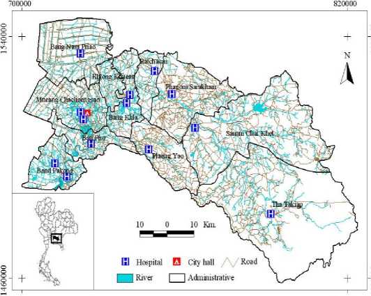
  Chachoengsao province had a morbidity rate of 39.68 per 100,000 population among provinces under the surveillance of the Ministry of Public Health of Thailand for 2007 (Table I). Chachoengsao, a province in the central part of Thailand, was selected as the study area (Figure 1). This province was selected as the study area because it has reported high incidence rates for the last several years. Chachoengsao province included 11 districts, which are Mueang Chachoengsao, Bang Khla, Bang Nam Prieo, Bang Pakong, Ban Pho, Phanom Sarakham, Sanam Chai Khet, Plaeng Yao, Ratchasan, Tha Takiap, and Khlong Khuean. The province is 80 km distant from the eastern part of Bangkok, and covers an area of 5,238.31 sq. km. The province has a population of about 645,022 people (Department of Administration, 2007).

TABLE I. TOP TEN MORBIDITY RATES OF DF/DHF/DSS INCIDENCE BY PROVINCE IN YEAR 2007

Rank	Province	Morbidity rate (per 100,000 population)
1.	Ranong	55.63
2.	Chachoengsao	39.68
3.	Saraburi	32.78
4.	Phetburi	31.78
5.	Prachinburi	30.15
6.	Ratchaburi	27.51
7.	Rayong	23.93
8.	Bangkok	23.42
9.	Nakhonphatom	23.12
10.	Lopburi	22.87

Source: Ministry of Public Health, Thailand

1540000                                                  1460000

700000                                                                              820000

Figure 1. Study area: Chachoengsao province, Thailand

• B.    Methods

The flowchart summarizes the methodology of the study as shown in Figure 2. Different components of the methods are detailed below:

1) Data Preparation

The study of spatio-temporal diffusion pattern and risk zonation of DF/DHF/DSS incidence covers the 821 villages in Chachoengsao province:

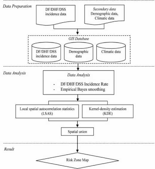
Figure 2. Methodology for mapping risk zones of DF/DHF/DSS

• a)    DF/DHF/DSS incidence data

  Chachoengsao province was selected for the case study because in every year, the incidence of DF/DHF/DSS has been high. DF/DHF/DSS data during years 2000 through 2007 were collected from the Chachoengsao Provincial Public Health Office, with regard to the number of reported cases per district per month, to record the probable and confirmed DF/DHF/DSS cases. Data represents only the patients who visit the hospital and fill the official Form 506 from the Bureau of Vector borne Disease, Ministry of Public Health, Thailand. The forms provided data such as the total of DF/DHF/DSS cases by month and year, type of disease, gender, and address of each patient. This data was employed for the study.

• b)    Demographic data

  The weekly data of the DF/DHF/DSS incidences in years 2001 and 2007, as they had high numbers of DF/DHF/DSS cases, and the total number of population by each village in year 2007 were also collected from Chachoengsao Provincial Public Health Office and Department of Administration, in order to deepen the observation and support the demographic aspect analysis. Some groupings were constructed, i.e., on the basis of the population distribution, age distribution, and gender using the data for year 2007 (Table III). Also, the classification by gender is presented in Table 2. Data analysis (Table II) revealed that the worst outbreak of DF/DHF/DSS cases took place in years 2001 (1,236 cases) and in 2007 (792 cases). Accordingly, data for these years were employed to define risk zonation in Chachoengsao province.

• c)    Climatic data

  Monthly weather data of rainfall, temperature, and humidity for the years from 2000 to 2007 were collected from the Department of Meteorology, Thailand. DF/DHF/DSS incidence outbreaks in Chachoengsao province occurred in years 2001 and 2007. The climate office has reported that that the DF/DHF/DSS incidence outbreaks coincided with El Nino years. El Nino events in Thailand are actually related to high temperature and also to low rainfall [2]. Thailand experiences rains from May to September. The remaining part of the year remains mostly dry. Besides the rainfall and temperature, humidity also influences dengue transmission [43]. Due to high humidity in rainy season, mosquito survival is longer and growth is conducive [44]. Overall, the temperature in Chachoengsao province was between 26.63 to 29.98°C in 8 years (2000-2007). Higher than 20°C is the favorable temperature for Aedes Aegypti mosquitoes [45]. The average monthly humidity in 8 years (2000-2007) was found to be 72.68%.

• 2)    Data Analysis

• a) Hotspot Delineation using Spatio-temporal Analysis

  It was found from data analysis that the worst outbreak of suspected DF/DHF/DSS cases happened in years 2001 (1,236 cases) and 2007 (792 cases). Thus those data were applied in this study to define hotspot and risk zonation during both years. The dengue (DF/DHF/DSS) incidence

rate ( IR Dengue ) is a ratio of number of observed incidence cases ( n i ) in each year divided by total population in each village ( p ). More explicitly;

^IRDengue ^{= ni                                       (1)}

p

In addition, hotspot analysis was carried out by using the empirical Bayes smoothing method, and dengue incidence rates were used to estimate underlying risk [46]. Concerning the empirical Bayes smoothing method, when raw rates are used to estimate this underlying risk, differences in population size result in variance instability and spurious outliers. So, rate smoothing is one way to address this variance instability. Essentially, rates are smoothed and thus stabilized by borrowing strength from other spatial units by using GeoDa 0.9.5i open source software [10,16,47] so all DF/DHF/DSS cases data in years 2001 and 2007 in Chachoengsao province were geocoded using GeoDa 0.9.5i and a custom address locator, which included village code. The 821 village locations were geocoded and saved in dBASE format. If choosing the latter, the counts for DF/DHF/DSS cases are usually standardized and compared with total of population distribution by villages for a total of 821 villages. Although this is a very common strategy, it is not always expected that the results are dependent on the configuration of area units. As a result, it has become common recently within studies of geographical epidemiology to conduct analysis that uses the point events themselves. Based on the local spatial autocorrelation statistics (LSAS) method, the hotspot of DF/DHF/DSS incidence analysis map was generated for 2001 and 2007 years in ArcGIS 10.

So to test for statistically significant local DF/DHF/DSS clusters for each year, and to determine the spatial extent of these clusters, the Getis-Ord G ^* statistic was used [34,48,49]. The G ^* statistic is useful for identifying individual members of local clusters by determining the spatial dependence and neighboring *

observations [49-51]. The G statistic includes the value at i in the calculation of G ^* . G ^* is calculated and then is output as the standard normal variant with an associated * probability from the z-score distribution [49,52]. The G is a group-level statistic, where point data must first be *

aggregated to areas. G was calculated using the spatial statistics tools in the ArcGIS 10 ArcToolbox.

Using the ratio of number of DF/DHF/DSS incidences in each village during years 2001 and 2007 divided by number of the population in each village in years 2001 and 2007, it was found that as many as 352 (2001) and 254 (2007) villages affected by DF/DHF/DSS incidence location at Chachoengsao matched the criteria to be the variables.

Moreover, the hotspot by using kernel-density estimation (KDE) method was carried out for finding the

DF/DHF/DSS incidence hotspot zonation map. Usually, the KDE is that the pattern has a density at any location in the study area. This density is estimated by counting the number of DF/DHF/DSS incidence cases in Chachoengsao province; centering the location where the estimate is to be made. The simplest approach, called the naive method in the literature, is to use a circle centered at the location for which a density estimate is required. KDE relates to location data and refers to a kernel method for obtaining a spatially smooth estimate of the local intensity of events over Chachoengsao province, which essentially amounts to a “DF/DHF/DSS risk zone” for the occurrence of those events.

DF/DHF/DSS incidence zonation maps were created using LSAS and KDE methods. The mean center or spatial mean gave the central location of disease points [53]. In this study, the UTM zone 47 North and WGS 84 coordinate system was adopted. With the coordinate system defined, the mean center can be found easily by calculating the mean of the x -coordinates (or Easting) and the mean of the y -coordinates (or Northing). These two means of the coordinates define the location of the mean center of DF/DHF/DSS incidence location as:

x mc , У те

V         7

nn h Sy n • n

V           7

Where x mc and y mc are the coordinates of DF/DHF/DSS incidence mean center, x i and y i are the coordinates of DF/DHF/DSS incidence in each point, and n is the number of points [54]. The incidence risk zones map was generated based on LSAS and KDE methods by using spatial union analysis.

• III.    Results and Discussion

  From documentation (Chachoengsao Provincial Public Health Office, 2007), it was found that DF/DHF/DSS occurred in the majority of the areas in Chachoengsao province; it inflicted severe health problems and financial tolls on the population affected. The worst outbreak of suspected DF/DHF/DSS cases was in year 2001 (1,236 cases) and in year 2007 (792 cases). The lowest occurrence was in year 2000 (380 cases). To widen the observation, the data collected from years 2000-2007 were classified into several groups for the ease of socioeconomic analysis, i.e. gender, area, timing, and age groups. Table II, shows that the total of cases reported was 5,565, composed of 2,989 males and 2,576 females. During the highest DF/DHF/DSS incidence in year 2001, male patients composed about 626 cases while female patients comprised only 610 cases. The ratio of male patients was higher than of female, which is 53.71%.

TABLE II. the number of df / dhs / dss cases classified by gender group from years 2000-2007

Year	Gender		Total
	Male	Female
2000	218	162	380
2001	626	610	1,236
2002	475	456	931
2003	374	316	690
2004	323	221	544
2005	306	217	523
2006	251	218	469
2007	416	416	792
Percentage (%)	53.71	46.29	100.00

Source: Chachoengsao Provincial Public Health Office

The climate of Thailand can be divided into three seasons: the hot season (February-May), rainy season (May-October), and cold season (October-February) respectively. Observation of the epidemiological characteristics of DF/DHF/DSS disease follows in three seasons. The distribution of DF/DHF/DSS incidence in years 2000-2007 is shown in Figure 3. Interestingly, disease patterns indicated that the critical months of incidence were during May to September, which is in the rainy season. The worst incidence noted was in July 2001 with more than 200 cases. The DF/DHF/DSS distribution in the whole province, having its highest incidence in rainy season, had a similar trend for every year. The cause of DF/DHF/DSS incidence is related to rainfall, temperature, and humidity so that DF/DHF/DSS generally occurred when the rainfall was comparatively lower and humidity was higher than average [2,55-57]. This demonstrates that rainfall, temperature, and humidity increased starting in May and after approximately 30 days or one month, the DF/DHF/DSS outbreak began. Moreover, in September, rainfall and humidity are highest.

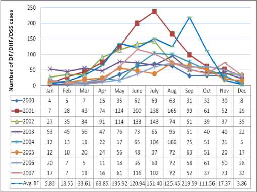
Figure 3. Number of DF/DHF/DSS cases and average rainfall on monthly basis from years 2000-2007

The monthly data was also broken down into a more detailed investigation. During year 2007, one of the highest outbreak years, 792 patients were suspected with DF/DHF/DSS cases. At that time, the epidemic took 20 weeks or 152 days, starting on 1st May and ending in high mobility of this population group on 31st September - in other words, the rainy season period. There were as many as 521 suspected DF/DHF/DSS cases spread throughout the region and it affected 0.08% of the total population (Figure 4). Approximately 25% of the cases occurred between Weeks 6-8, with the highest number occurring in Mueang Chachoengsao district of which 178 cases were reported, and the second highest was Panom Sarakham district with 170 cases. Most cases happened in June 2007, with 171 cases, while February 2007 had the lowest rate with only 9 cases.

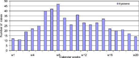
Figure 4. Number of suspected DF/DHF/DSS cases reported weekly during the 2007 epidemic (May 01-September 30)

Disease distribution based on age of the patients was also determined. The age distribution of DF/DHF/DSS cases was different from the population age distribution and the highest incidence was in the 13 to 24 year group and percentage rate of incidence was 42.9%, with a lower incidence on population older than 25 years old and percentage rate of incidence was 24.3% (Table III).

TABLE III. T he number of DF/DHF/DSS cases by age group distribution for year 2007

Age group (year)	DF/DHF/ DSS (case)	Total population 2007	Rate of DF/DHF/DSS Incidence (%)	Population Rate (%)
0-12	260	117,194	32.8	18.2
13-24	340	118,823	42.9	18.4
25-36	121	132,832	15.3	20.6
37-48	52	126,104	6.6	19.5
> 48	19	150,069	2.4	23.3
Total	792	645,022	100.0	100.0

Source: Chachoengsao Provincial Public Health Office

All spatial statistics processing to create hotspots was carried out using the spatial statistics tools in the ArcGIS 10 ArcToolbox. The hotspot analysis was carried out using the “Hotspot Analysis (Getis-Ord G ^* )” tool in the mapping cluster tools extension. By plotting the hotspots of outbreaks in years 2001 and 2007, the zonation was found to be along the Bang Pakong River (Figure 5).

A DF/DHF/DSS incidence map was constructed from the cumulative number of cases during the entire epidemic, and confirmed that DF/DHF/DSS cases were spreading all around the province with hotspots in the Mueang Chachoengsao (2001) and Panom Sarakham (2001 and 2007), and were around the urban centers (Figure 6).

The mean center of the cases were found in critical months, especially during rainy season from May through September in years 2001 and 2007 (Figure 7). It also showed the trend diffusion cluster pattern in the center of the province at Bang Khla district.

From Figure 8, it can be concluded that movement from location 1 (May) to location 2 (June) moved to the east in 2001 but moved to the west in 2007, and changed direction to the west to location 3 (July) in 2001 but moved to the north in 2007 and moved to location 4 (August) in the north and changed direction to location 5 (September) in the west, same as year 2007. This kind of recording is necessary for agent-based models as implied in our study of pedestrian disease in space and time.

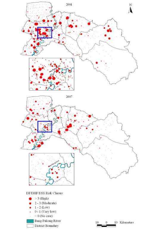
Figure 5. Incidence maps showing the hotspot distribution of DF/DHF/DSS outbreaks during the years 2001 and 2007 using local spatial autocorrelation statistic (LSAS) method

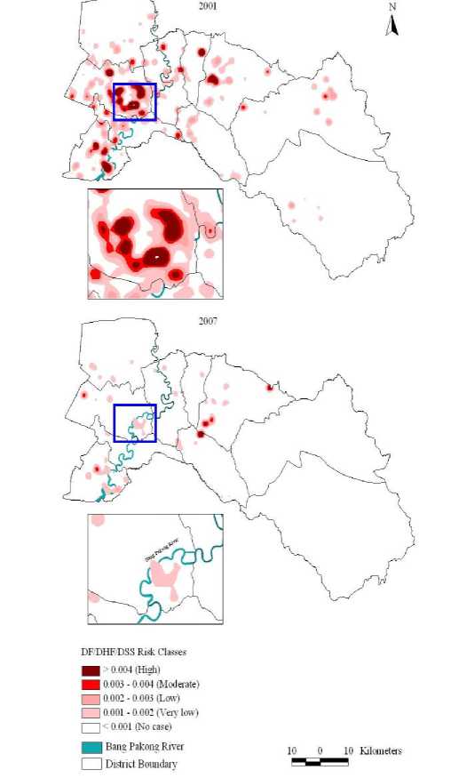
Figure 6. Incidence map showing cumulative number of DF/DHF/DSS cases in 2001 and 2007 outbreaks using kernel-density estimation (KDE) method

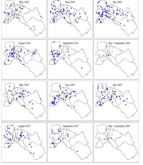
Figure 7. The mean center locations of DF/DHF/DSS outbreaks between May-September in years 2001 and 2007

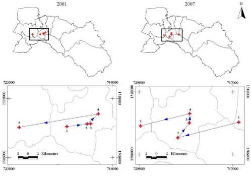
Figure 8. Temporal dynamics in space and time. The mean center locations of DF/DHF/DSS outbreaks between May-September (1 → 2 → 3 → 4 → 5) in years 2001 and 2007

Lastly, Figure 9 represents the DF/DHF/DSS risk zone map in Chachoengsao province by spatial union analysis.

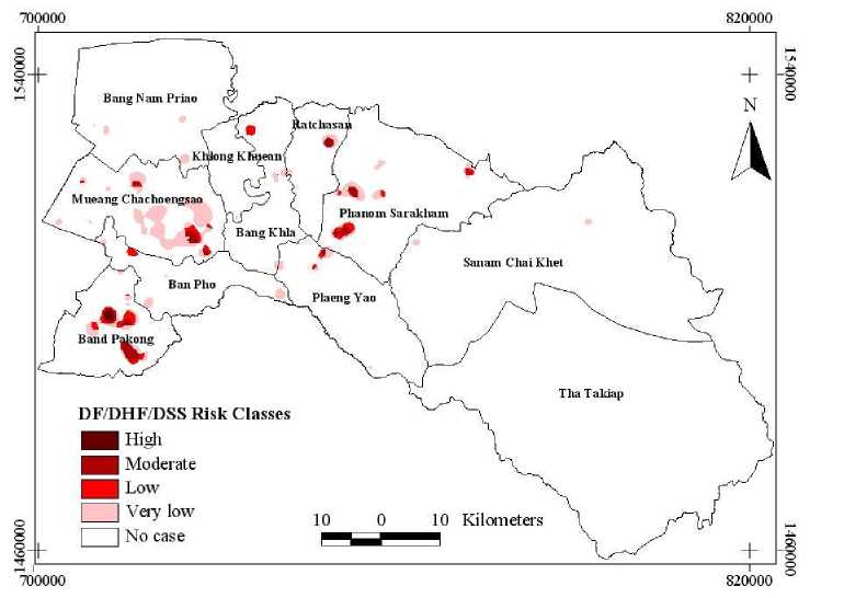
Figure 9. DF/DHF/DSS risk zone map of Chachoengsao province, Thailand

Table IV shows the summary of DF/DHF/DSS risk zones with the total number of villages (821 villages). Results indicated that the highest risk zone covered 7 villages (0.85%, 2.45 km2 of total area), the moderate risk zone comprised of 39 villages (4.75%, 23.49 km2 of total area), the low risk zone of 22 villages (2.68%, 26.07 km2 of total area) was found, the very low risk zone consisted of 120 villages (14.62%, 111.49 km2 of total area) and no case consisted 633 villages (77.10%, 5074.81 km2 of total area).

TABLE IV. S ummary of villages DF/DHF/DSS affected

Risk classes	DF/DHF/DSS affected	Percentage (%)	Area (km 2 )
High	7	0.85	2.45
Moderate	39	4.75	23.49
Low	22	2.68	26.07
Very low	120	14.62	111.49
No case	633	77.10	5074.81
Total	821	100.00	5238.31

• IV.    Conclusion

  Recent monitoring and planning of control measures for dengue epidemics have become a critical issue. This research offered useful information relating to the DF/DHF/DSS incidences. To analyze the dynamic pattern of the 2001 and 2007 DF/DHF/DSS outbreaks in Chachoengsao province, Thailand, all DF/DHF/DSS cases were positioned in space and time by addressing the respective villages.

This takes into account that the quite high incidence of DF/DHF/DSS cases were in the age group of 0-24 years old. It was also noted that males have a higher risk of incidence than females. Thanks to awareness amongst older people, the prior immunity to dengue in older individuals, and less mosquito biting rates in children, there are less numbers of victims in other age groups. Meanwhile, the mobility of productive aged people within “hotspot” neighborhoods has led them into the risk of getting infected with DF/DHF/DSS. Analysis of the climatic factors such as rainfall, temperature, and humidity with the dengue incidences has shown that dengue generally occurred when average temperature rose above normal, and also occurred when the humidity was higher than average and rainfall was reasonably lower. In 2007, the Chachoengsao Provincial Public Health Office reported 792 suspected DF/DHF/DSS cases and a total of 171 DF/DHF/DSS cases occurred in June. During the 152 days of the epidemic, there were as many as 521 suspected DF/DHF/DSS cases spread throughout the region and affected 0.08% of the total population. Furthermore, several studies confirmed that dengue risk exposure is greater at home because of endophilic habits of Aedes Aegypti and clinical symptoms may also be less reported in young people because of better self-recovery ability [11] .

Spatial autocorrelation can be a valuable tool to study how spatial patterns change over time [58]. The empirical Bayes method has the technique to improve the population density from IR Dengue to be empirical Bayes rate which is more accurate and useful. This theorem enables researchers to analyze population data and whatsoever by determining the total of DF/DHF/DSS cases with the number of population per village each year.

Based on the local spatial autocorrelation statistics (LSAS) method, the hotspot of DF/DHF/DSS incidence analysis map was generated for 2001 and 2007 years by using the spatial statistics tools in the ArcGIS 10 ArcToolbox software. Moreover, the kernel-density transformation is one of the most useful in applied GIS analysis. First, it provides a very good way of visualizing a point pattern to detect hotspots. Second, since it produces a map of estimates of the local intensity of any spatial process, it is also a useful way to check whether or not that process is first-order stationary. A first-order stationary process should show only local variations from the average intensity rather than marked trends across the study region. Third, it provides a good way of linking point objects to other geographic data [59]. KDE method is used to obtain spatially smooth estimates of the local intensity of points of DF/DHF/DSS cases by village locations in years 2001 and 2007 (Figure 6). The function gives the value of λ for a specified point pattern, evaluated over a grid of locations that span a particular polygon. The width of the kernel is specified by average distance of flying dengue mosquito of 2 kilometres. One useful display is a raster image [60]. The mean center of disease was shows cluster pattern in the center of the province, Bang Khla district, and also shows how the mean center locations of disease changed in space and time by movement of location 1 to location 5 (May to September) in years 2001 and 2007. The spatial statistics are used to summarize the description of a set of locations, followed by measures indicating the directional biases of a set of points. The DF/DHF/DSS risk map obtained from the research is able to support public health officers in space and time so as to control and predict dengue spread over an extension area. Moreover, the risk map can be beneficial for public warning and awareness. Public health officers may employ the model to control DF/DHF/DSS distribution and hotspots through factors mentioned above. Not only it is applicable in epidemics, but this model is general and can also be applied in other application fields such as outbreak of other diseases during natural disasters.

• V.    Acknowledgements

I would like to express my sincere gratitude to School of Information and Communication Technology (ICT), University of Phayao, Thailand for providing financial support to this study. Special thanks to Chachoengsao Provincial Public Health Office, Department of Administration, Department of Meteorology, Thailand for data and information.