Spiking neural network and bull genetic algorithm for active vibration control

Published Online February 2018 in MECS

One of the major real problems faced by all types of flexible structure systems is the vibration that may cause them to fail or damage. To tackle this problem, many traditional methods have been used. It includes a passive control, where a passive material is mounted on the structure [1-5]; and many Active Vibration Control (AVC) techniques, where cancelling sources are generated by artificial means to deliver destructive interference with the unwanted source. It reduces the level of vibration or disturbances occurring at the desired site.

In order to observe the AVC system for identifying its features, a model for the flexible structure system using system identification schemes is required. The parameters of this model should be adjusted until the actual outputs match the measured outputs. A model for the system is highly essential for analyzing, simulating, predicting, monitoring, diagnosing, and controlling the system design. The conventional approaches for the system identification usually are failed to look for the global optimum.

Conventional methods are often used for searching the global optimum in the system identification. These approaches often fail, especially in the instance of nonliner search space related to the parameters. Many bioinspired and artificial intelligent techniques have been addressed to overcome these limitations [6-16]. In this paper, Bull Genetic Algorithm (BGA) and the spiking neural networks have been utilized to identify the properties concerning the system identification and AVC for a flexible beam system. The test platform employed a model based on the flexible beam system with transvers vibration. These kinds of systems can have numerous modes, where most attention is required by the lower modes. This paper has assumed that the unwanted vibrations occurring within a structure are primarily produced because of the disturbance of a single point possessing wideband nature. For addressing the beam behaviors, developing a relevant test and verifying the platform, the study used the first-order central finite difference (FD) method [4]. The design of AVC system is based on a control system that has one input and one output. The structure assists in achieving the optimal cancellation of broadband vibration that may arise within the observation points along the beam. BGA and spiking neural network are used to evaluate the AVC systemcanceling signal on the basis of input and resultant output generated from the flexible beam model. The vital role of suggested approaches is to minimize the error between the output collected from the actual plant and its corresponding model. The paper is organized as follows. Section 2 gives the bull genetic algorithm. Section 3 introduces spiking neuro network. Section 4 presents active vibration control. Section 5 presents experiments and discussions. Section 6 demonstrates identification algorithms impact on the control system design. Section 7 concludes the paper.

• II.    Bull Genetic Algorithm

The Bull Genetic Algorithm (BGA) is known to be an enhanced version developed from the traditional genetic algorithm. It is recognized as a contemporary medium of population-based search algorithm, which can implement a new naturally selection process, inspired from the bull in cattle. It has a new structure of individuals (population) and a different reproduction type that simulate the structure of diploid and the reproduction process of multicellular organisms [17-19].

The modality of BGA employs the crossover operation where it actively uses the best individual for producing an offspring. The results of crossover compete to attain improvements by adopting the excelling features of best entity. At initial stages, the offspring undergo mutations for varying times, until the best outcomes are achieved. These mutations can also be seized if the number of experiments reached the limitation. The primary objective of BGA is producing individuals better than those who were in the initial phase. Creation of random individuals is kept limited to the initial stages while other stages are only carried out to more improvement.

In BGA, the nature simplest approach to represent gens is to use binary encoding using only two alleles to represent the gens where:

• 0: Encoding gene 0.

• 1:    Encoding gene 1.

However, in some applications, it provides better performance, ease of implementation, and flexibility to represent the gens with more than two alleles. Table 1 shows dominance map with three alleles per gene.

Table 1. Dominance map with three alleles per gene

Alleles	0	1	2
0	0	0	1
1	0	1	1
2	1	1	1

Where

• 0:    Encoding gene 0.

• 1:    Recessive encoding for gene 1.

• 2:    Dominant encoding for gene 1.

In case of using logical OR function, then allele (1) is the dominant allele while in case of using logical AND function, than allele (0) is the dominant allele.

For example, if there are eight genes for each individual, the alleles to represent parents and the offspring are as shown in table 2.

The offspring will randomly select its genes from both parents as in Meiosis. The main idea is that, the offspring will inherit about half of their genes from their father and the other half from their mother. According to these concepts, BGA is different from the traditional GA in four ways:

• 1.    BGA mating pool is considered cattle and its bull is the individual with the best fitness, the rest are females; but in GA, individuals are selected randomly.

• 2.    BGA constructs the offspring by reproducing the only one male (bull) with each one of the rest (females),

• 3.    BGA individual structure is diploid not haploid.

• 4.    BGA matting type is meiosis as in complex live forms not mitosis.

not randomly between individuals.

Table 2. Dominance map with binary encoding per gene

Parent1
1	0	1	0	1	1	0	0
0	0	1	1	1	0	1	1
Parent2
0	0	1	1	1	0	0	0
1	1	1	0	1	0	1	1
Offspring
0	0	1	0	1	0	0	0
0	1	1	0	1	0	1	1
If allele (1) is the dominant gene, then the child is expressed as follows:
0	1	1	0	1	0	1	1

The developed BGA pseudo code is written as follows:

• 1.    Generate a population randomly of N individuals, each having diploid chromosomes.

• 2.    Evaluate individuals in their expressed form (apply dominance on genes) to get record the fitness.

• 3.    Categorize the recruited individuals from the selected random population in accordance to the fitness.

• 4.    Select the best N individuals and deploy them for the mating pool.

• 5.    Choose the best individuals according to their fitness -      as      the      male      (bull)      and     rest

• 6.    Produce new line of N-1 individuals by mating the bull with all of the females producing only one child for each female.

• 7.    Apply mutation operation.

• 8.    Repeat step 2-7 for the best fitness value.

N-1 as females (cows) for producing a new population.

• III.    Spiking Neural Networks Architecture

The architecture of the spiking neural networks (SNNs) appears to be parallel to the traditional neural networks. The architectural difference is attributed to the synaptic terminals located between each layer of neurons and delay in synapses. The behavior of spiking neurons has been described by many proposed mathematical models [20-21].

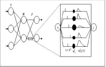
Fig.1. Spiking neural network with feed forwarding and multiple synaptic terminals.

The model is composed of a spiking neural network in connection with a feed forward that delivers multitude synaptic terminals with delay. The labels on the structure have been called I for input, H for hidden, and J for the output layers, figure 1 has demonstrated the model. The relationship between the spikes from the input and the variables of internal state have been described with the spiking neurons. These spiking neurons were adopted on the basis of the Spike Response Model or SRM [20]. In this approach, a neuron j is considered with a set of immediate pre-synaptic neurons known as D j . The neuron receives a set of spikes with firing times defined as t i , i g D j . It is presumed that a neuron is able to produce one spike more likely, during simulation interval, and can deliver when the variable of the internal state attains the threshold. The dynamics of internal state variable y ( t ) can be defined as:

у , ^{( t} ) = Т , D w * x j ^{( t} ) . (1)

Where x_j ( t ) in this equation expresses the unweighted contribution that is delivered by a single synaptic terminal towards the state variable y ( t ). The expression can be described as a pre-synaptic spike that is generated at the synaptic terminal k, with the use of a post-synaptic potential (PSP) as:

y k = ^ ( t - t i ^- d^k ) ■ ⁽²⁾

Where the time t in this equation indicates the time of pre-synaptic neuron firing. The synaptic neurons are expressed as i. Delay in synapse is presented by d^k while k represents the synaptic terminal In case of multiple synapses within a connection, the state variable y j ( t ) of neuron j is known to receive numerous inputs from all other neurons in the preceding network. The expression describes the weighted sum of the pre-synaptic contribution as:

m yj (t) = S„D Swki * xk (t) (3) j k=1

Where e ( t ) is the spike response function that describes the effect generated by the spikes from the input while w weights the synaptic strengths. In order to implement a leaky-integrate-and-fire spiking neuron, the spike response function e ( t ) is demonstrated with a - function:

1 - -                               ,.

e ( t ) = — e ^T , for t > 0, else e ( t ) = 0.        (4)

т

Where τ is the time constant that describes the postsynaptic potential (PSP) in terms of rising and falling of the time. An individual connection is composed of a fixed number of synaptic terminals. Every terminal tends to serve as a sub-connection. Each sub-connection is known to be in connection with different delays and weights. The delay of a synaptic terminal k defines the difference that occurs between the time of firing from a pre-synaptic neuron and the initiation time of the rise of post-synaptic potential. The threshold is considered constant and is donated by θ that remains equal throughout the network for every neuron.

• A. Spiking neural network for supervised learning procedure

The work has been performed on the supervised learning [20] that aimed to improve the supervised learning algorithm known as the SpikeProp, which looks like the traditional back propagation error algorithm. The algorithm objective is to learn a group of target firing times that occurs at the output neurons for a provided set of input patterns. In this model, the variables are denoted by the following expressions:

Target firing times:{t^d_j } Output neurons: j g J

Input pattern: {P[t ₁ , t ₂ ,..., t_i ]}

Where {P[t , t ,..., t ]} is single input pattern occurring in response to the single spike-times for each neuron i g I .

The error function is considered as the least mean square error. With the actual firing times { t^a } and desired spike times { t^d }, the error-function is expressed as:

E = 1 S j ⁽ t a - t: d) ■ (5)

As derived by the connection’s weight, the general form of error is:

®L = 5 E ( t a )2 ti_ ( , a ) д 0^ ( , a )

d w ik   5 tj^Vj ’ aa j ( t^j) d w k

= e i ( t a - t a - d a ) .                   (6)

In this expression, 8j for neurons in output layer ^ 8j for neurons in the hidden layers.

Where

Г j direct pre-synaptic neurons j

Г ^j = neuron j direct successors.

An equation for output layer neuron is defined as:

⁰ j =

- (a - j

k

У Vw k -Це-td-dkX

L .L wj St t j ^{4 d}ij

An equation for hidden neurons h e H, — is defined as:

- =

k

У   - У w k    ( t ^J - A - d k )

Z^I erj - Z—ik -j -t    1    -      lJ k.

E X' k ⁰⁸ ij  a d k

- er j L-- ^{( t}J — t - — j

Error backpropagation is evident in these expressions as 0 j tends to be relied on all 8 j 's of the neuron j successors. The adaptation rule for the weights is expressed as:

w j ( T + 1 ) = w -j ( T ) +A w j ( T ) •           (9)

Where T = Tth is the step of the algorithm which expresses the simulation interval wnew  wnew + A w-j (T).            (10)

A w -j ( T ^"d^-"" ( T ) . ° w ij

Where η is the learning rate. The error is minimized by creating a change in the value of the weights using the negative local gradient.

• IV.    Active Vibration Control (AVC)

AVC is an old concept which has been proposed on the basis of principles presented for the cancellation of noise [1–2]. In order to void the disturbances created by the unwanted vibrations within a structure, many researchers have attempted to develop methods that can tackle the resulting outcomes. These disturbances are reduced using active and passive control [5]. Traditional approaches that have been employed to suppress the vibration have included the methods like passive control. The passive control involves the mounting of passive material on the model [2]. On contrary, AVC is composed of cancelling sources that are generated from the artificial means. These sources interfere with the unwanted sources of disturbances in a destructive manner. Ultimately, the level of disturbing vibrations is reduced at the desired site. The cancellation is attained when the detected and processed vibration developed from a suitable means of electronic controller is superimposed with the disturbances. The control mechanism must realize suitable characteristics for the frequency dependency and able to cancel the range of frequencies within the system at which the most disturbance occur. The whole idea entails that the control mechanism should be efficient in order to identify and locate the disturbances within a system that is needed to achieve and manage the desired level of performance [1-4].

The performance evaluation of learning algorithms requires an investigative platform. The platform is the simulation model of cantilever beam in the transverse vibration. When exposed to the disturbance forces, the flexible structure systems tend to exhibit inherent property of vibration. These vibrations lead to the damage of either a component or structural damage, or both. The flexible beam and the associated control system of the active vibration are utilized as the platform for case studies that may employ GRNN, BA, and/or GAs [6-15]. In this section, a cantilever beam is presented as shown in figure 2, which is considered with the following characteristics:

Where L : Cantilever beam length,

U(x, t): Supplied force, x : Distance at which the force is applied at the fixed end, t : The time at which the force is applied,

^{y (} x , t ) : The resultant deflection of the beam from the stationary position. The position is located at the point of force application.

Using partial differential equation with fourth order governs the beam motion in the transvers vibration [4-5].

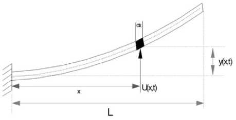
Fig.2. Cantilever beam system. [4]

2 94У (X, t)   92 y (x, t)   J_ dx4        dt2     m

Where, Ц =Beam constant, given by

2    ^EI

^ =^—л , PA

p = Mass density,

A = Cross-sectional area,

I = The beam moment of inertia,

E = Young modulus, m = Mass of the beam.

At the sites of fixed and free ends of the beams, the conditions of corresponding boundary are expressed as:

y ( 0, t ) = 0.       and     ^^^’ t^ = 0.

v 7cX d 2 y ( L, t)                 d 3 y ( L, t)

= 0. and= cX 2c

The models indicate that there has been no damping incorporated. For constructing a testing platform, a method is needed to be adopted for achieving a numerical solution for equation (12). It requires the utilization of finite difference (FD) method. It also involves the discretization of beam. The beam is divided into bounded number of equal-length segments. The characteristics are expressed as:

^А = length of the beam,

^A t = duration of equally spaced time, in which length of the beam are deflected for each section.

Eventually, the first-order central FD methods approximate the partial derivative terms in the given equations (12) and (13).

Y j _{+ 1} = - Y j - 1 - 2 2 SY j + ( A t ) 2 U ( x , t ) — .  (14)

m

Where yk : n x 1 Matrix shows the beam deflection grid-points 1 to n , k : Deflection time,

S : Matrix represents the beam features and the steps of discretization,

A t , A x , 2 are discretization steps.

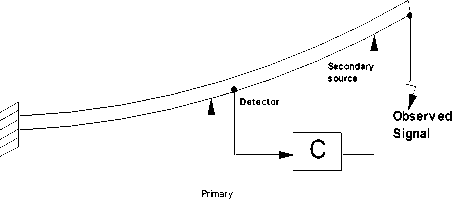
Equation (14) characterizes the particular behavior displayed by the cantilever beam system. The behavior of the beam system can be easily implied on a digital computer. A necessary and sufficient condition for stabilizing the convergence requirement is displayed as 0 <  2 <  0.25 [1]. Figure 3 represents a system with the signals: U = input, and Y = output.

The represented system allows the development of an AVC algorithm. In the given equation, the signal Y is forced to reach zero for cancelling the disturbance at the observation point. The approach displays a requirement for the primary and secondary signals at the observation point, which are the same in the magnitude and demonstrates a phase shift of 180 ^o in relation to one another.

source

Fig.3. The structure of AVC System

• V.    Experiments and Disccuions

For demonstrating the ability of spiking neural network and bull genetic algorithm for a system identification algorithms, FD method is used and a simulation platform of a flexible beam system in transverse vibration is considered. Although, lower modes act as dominant ones in most cases that require attention, a system displays numerous modes. A simulated beam presents a number of specifications that include:

• •    The beam Length, L, is specified at 0.635 meters

• •    The beam mass, m, is specified at 0.037 kg, and

• •    The constant of the beam, ц, is specified at 1.351

As obtained by the conducted simulated experiments and confirmed through the theoretical analysis, it has been noted that the initial five resonance modes of the beam are positioned at the following frequencies: 2 Hz, 12 Hz, 33 Hz, 65 Hz and 107Hz respectively. Among these, the first and the second frequencies are considered as the dominant modes. The beam is further divided to twenty small sections. Along the model, a time interval A t = 0.3 ms is chosen. It aims to satisfy the stability requirements of FD simulation algorithm (Equation 14) which is sufficient for all modes of resonance in the beam vibration. For the purpose of attaining stability, X is chosen equal to 0.36 [4]. In order to generate excitation in the dominant modes of the beam vibration, 0.1N disturbance force step is chosen with a limited period of 0.3ms to be employed as an initial force at point 16 of the grid. Whereas, a control actuator signal is provided at the grid point 20. Furthermore, a sensing device, sensor, or detector along with an observer is placed at gird points 16 and 20, respectively. Both of the modalities are planted as the input and output samples. The following equation has been selected to represent the flexible beam system as a linear discrete second order mode:

Y ( z ) = b^{0 +} bz -' ⁺ b ² z -² U ( z )         (15)

• 1    + a 1 z  + a 2 z

The system identification experiments have been performed for around 5 seconds (16,700 iterations) by employing the equation (15) at both point 16 and point 20 of the grid. The data input sets and data output sets have been simulated by using the equation (14). BGA estimates the parameters provided in the model using equation (15). Furthermore, spiking neural network estimates the equivalent model that uses the plant input as well as its corresponding output. It is worth noting that, a set of 16,700 pairs of actual input (grid point 16) and output (grid point 20) was generated using equation (14). The spiking neural network is then practiced by the use of this set of data.

• A.    System Identification Performance of the Proposed Algorithms in Time Domain

This section presents the beam actual fluctuation as observed at the end point and the estimated beam fluctuation at the end point using different algorithms. The fluctuation has been measured for 5 sec and figure 4 displays BGA’s time domain performance along with the spiking neural network and the actual output. It has been clearly observed that a substantial degree of convergence have be obtained using both approaches even BGA outperforms by 7%.

• B.    Algorithms in an auto-power spectral density

Figure 5 presented a frequency domain performance of the proposed algorithms that showed a remarkable convergence between actual and estimated outputs in frequency domain using BGA and SNN. The estimated outputs of proposed approaches are almost tracking the actual output, and BGA has better performance compared with SNN with 3%. Equation 16 expresses the error that has been estimated based on the absolute value of the difference observed between the actual output signal and estimated output signal.

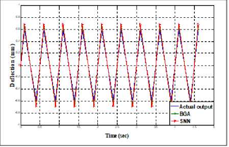
Fig.4. Achieved performance in time domain using BGA and SNN

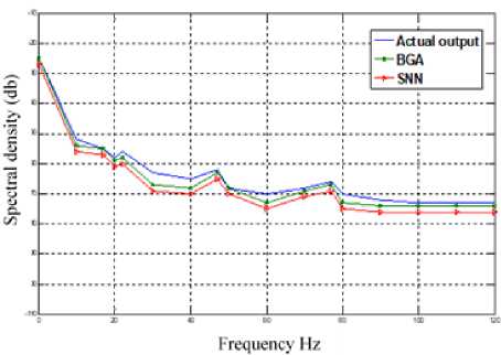
Fig.5. Frequency domain performance of the proposed approaches

L y (k ) - y (k )| f (e) = 100* k=1-r--------- (16)

L y ^{( k} ) k = 1

Where, y = actual output, y ˆ = estimated output.

• VI. Identification Algorithms Impact on the Control System Design

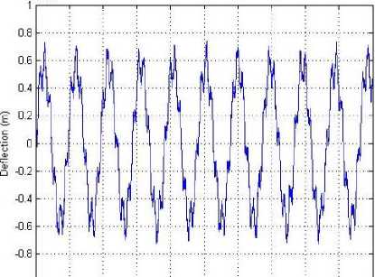
Since BGA algorithm estimates the AVC system parameters using input-output plant model. On the other hand, AVC system model using SNN has been established on the basis of input and the cancellation signals. The cancelling signals are primarily required for the destructive interference at the point of control. It is clear that 180o phase shift of an output signal is considered as the signal of cancellation. On the basis of prior examination and as addressed in system identification section, sites of the input sensing device, sensor, and the output device, actuator, are chosen for the efficient behavior. The AVC system has been tested and validated after conducting a set of simulated experimentations. Figure 6 displays the system response before cancellation in time domain at the end point of the beam fluctuation. Similarly, figure 7 and figure 8 show resultant vibration after cancellation using BGA and SNN approaches. It has been identified in the identification section that BGA offers better convergence than SNN algorithm. The approach helps to locate parameters that can be more accurate controller and give better presentation compared with SNN in implementing the AVC system.

_■] _______________________I_______________________I________________________I_______________________I________________________I_______________________I_______________________ I________________________ I_______________________I________________________

0     0.5     1     1.5     2     2.5     3     3.5     4     4.5     5

Time (s)

Fig.6. Fluctuation in the beam before disturbance cancellation

Fig.7. Fluctuation in beam using BGA

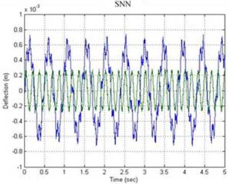
Fig.8. Fluctuation in beam using SNN

• A.    Performance of 3-D time domain along the beam length using intelligent algorithms prior to and following the cancellation

Figure 9 shows suppression of vibrations in a 3-D time domain prior to the cancellation. The corresponding suppression of the vibration with the implementation of AVC system is displayed in figure 10 and figure 11 for BGA and SNN approaches respectively. It has been noticed that a remarkable degree in the suppression of the vibration is attained through BGA algorithm at the end point and along the length of the beam. Moreover, a minor fluctuation has been seen at the middle of the beam length.

• B.    Fluctuations in time domain lateral to the 2D grid points

Figure 12 presents the whole range of fluctuations observed along the beam length. In this figure, the dotted line depicts the deflection with the minimum value and maximum value along the points of the grid prior to the cancellation. Furthermore, solid lines display the deflection amplitude using BGA and SNN algorithms at the period of random sampling.

It is shown that the beam fluctuation range after cancellation using both BGA and SNN remains almost the same.

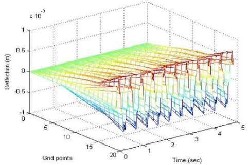
Fig.9. Fluctuation in beam along the length prior to the cancellation

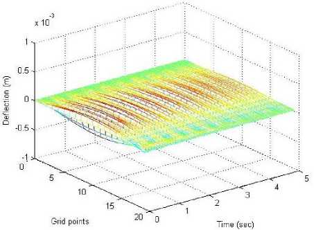
Fig.10. Fluctuation in beam along the length following the cancellation with the implementation of AVC using BGA

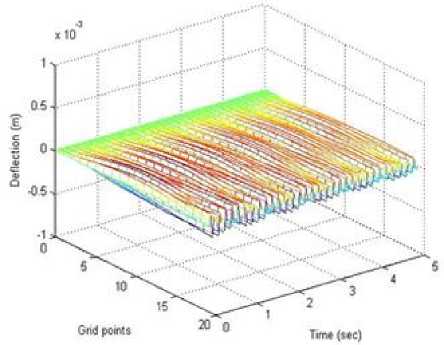
Fig.11. Fluctuation of beam along the length following the cancellation with the implementation of AVC using SNN

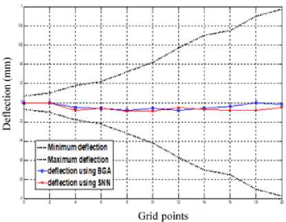
Fig.12. The beam fluctuation range before and after cancellation using BGA and SNN algorithms

• C.    Auto-power spectral density (in db)

Figure 13 presents the auto-power spectral density (in db) that is located at the beam end point. It displays the auto-power spectral density prior to the suppression of the vibration. Moreover, the cancellation of vibration with the implementation of the AVC system is displayed in Figure 14 and figure 15 by the use of BGA and SNN respectively. The auto-power spectral density prior to the cancellation is denoted by solid lines; while it displayed after the cancellation by the dotted lines. A considerable degree of drop is attained via BGA for the initial resonance frequency. Based on the achieved results, it is observed that the overall energy level following the cancellation for all resonance frequencies by the use of AVC system reduces. Furthermore, BGA achieves better performance in lower frequencies than SNN. Based on all experimental results and convergence analysis achieved, BGA consistently performed better than SNN. Both proposed artificial techniques, BGA and SNN, achieved better performance as compared with most approaches. For qualitative comparison, the proposed approaches have been compared with the related approaches and table 3 summarizes the achieved results.

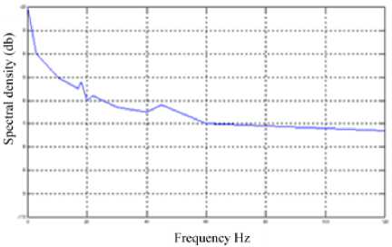
Fig.13. The beam fluctuation range before cancellation

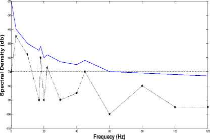
Fig.14. The beam fluctuation range after cancellation using BGA

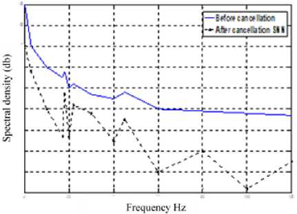
Fig.15. The beam fluctuation range after cancellation using SNN

Table 3. Performance comparison among different heuristics approaches AVC

Algorithm	Normalized Error
RLS	20.24
ANFIS	19.93
GA	19.86
GRNN	19.74
BA	19.69
SNN	19.14
BGA	18.52

• VII. Conclusions

This paper presented two heuristic approaches; bull genetic algorithm and spiking neural network for active vibration control. For testing and validating, a flexible beam system in transverse vibration is considered as an investigative platform. In order to validate the competences and merits of the learning algorithms, AVC system has been selected for the implementation and verification over a determined set of experimentation. A comparative practice in applying the AVC system using RLS, ANFIS, GA, GRNN, BA, SNN, and BGA has been presented and discussed. The comparative study has shown that the proposed approaches outperformed other intelligent learning algorithms; especially BGA because it has a good selection approach with a better way of population inheritance using the bull concept.

Refeernces

• [1]    A. R. Tavakolpour, “Mechatronic Design of intelligent active vibration control systems for flexible structures,” PhD Thesis, Faculty of Mechanical Engineering, university of technology, Malaysia, 2010.

• [2]    A. Madkour, M. A. Hossain, K. P. Dahal, Y.Yu, “Intelligent learning algorithms for active vibration control,”   IEEE Trans. on Systems, Man, and

  Cybernetics—Part C : Applications and Reviews, Vol. 37, No. 5, 2007, PP. 1022-1033.

• [3]    K. Andrzej, “Desiginig of active vibration control system for smart structure 2-D with non-collocated piezoelements,” 22nd Int. Conference on Methods and Models in Automation and Robotics (MMAR), 20 17.

• [4]    B. Nossair, A. Madkour, M. A. Awadalla, and M.M. Abdulhady, “System Identification Using Intelligent Algorithms,” Int. conference on aerospace sciences and aviation technology , 2009.

• [5]    J. Fei, “Adaptive sliding mode vibration control schemes for flexible structure system,” IEEE Conference on Decision and Control 2007, New Orleans (USA).

• [6]    A. Ali, M. A. Tawhid, “A hybrid particle swarm optimization and genetic algorithm with population partitioning for large scale optimization problems,” Ain Shams Engineering Journal , Vol. 8, Issue 2, 2017, PP. 191-206.

• [7]    M. Awadalla, A. Elewi, “Enhanced PSO Approach for Real Time Systems Scheduling,” Int. journal of Computer Theory and Engineering , Vol. 8, No. 4, 2016, PP. 285-289.

• [8]    A. Khare, S. Rangnekar, “A review of particle swarm optimization and its applications in solar photovoltaic system,” Applied Soft Computer , 2013; 13, PP. 2997-3006.

• [9]    L. Hongqiang, Y. Danyang, M. Xiangdong, C. Dianyin, C. Lu, “Genetic algorithm for the optimization of features and neural networks in ECG signals classification, ” Sci Rep . 2017; 7: 41011.

• [10]    W. R. Mebane, J. S. Sekhon, “Genetic optimization using derivatives," Journal of Statistical Software , Vol. 42, No. 11, 2011, PP. 1-26.

• [11]    H. Nagham H. Saeed, F. Maysam, “Modelling Oil Pipelines Grid: Neuro-fuzzy Supervision System,” Int. Journal of Intelligent Systems and Applications(IJISA), Vol. 9, No. 10, Oct. 2017.

• [12]    J. Ban, C. Chang, “The learning problem of multi-layer neural networks,” Neural Networks , Vol. 46, 2013, PP. 116-123.

• [13]    Y. Bodyanskiy, O. Vynokurova, V. Savvo, T. Tverdokhlib, P. MulesaHybrid, “Clustering-Classification Neural Network in the Medical Diagnostics of the Reactive Arthritis,” Int. Journal of Intelligent Systems and Applications (IJISA) , Vol. 8, No. 8, Aug. 2016.

• [14]    M. Awadalla, H. Yousef, “Neural Networks for Flow Bottom Hole Pressure Prediction,” Int. Journal of Electrical and Computer Engineering (IJECE) , Vol. 6, No. 4, August 2016.

• [15]    Nidhi Arora, Jatinderkumar R. SainiEstimation and Approximation Using Neuro-Fuzzy Systems,” Int. Journal of Intelligent Systems and Applications(IJISA), Vol. 8, No. 6, Jun. 2016, PP.9-18.

• [16]    S. Lalwani, S. Singhal, R. Kumar, and N. Gupta, “A comprehensive survey: applications of multi-objective particle swarm optimization algorithm,” Trans. on Combinatorics, Vol. 2, No. 1, 2013, PP. 39-101

• [17]    B. Shu-Nong, “The concept of the sexual reproduction cycle and its evolutionary significance,” Plant Science , 2015, pp 6-11.

• [18]    R. K. Sherwood, C. M. Scaduto, S. E. Torres, R. J. Bennett, “Convergent evolution of a fused sexual cycle promotes the haploid lifestyle,” Nature , Vol. 506, No. 7488, 2015, PP. 387-390.

• [19]    A. L Hodgkin, A. F Huxley, “A quantitative description of membrane current and its application to conduction and excitation in nerve,” Journal of Physiology , Vol. 117, No. 4, 1992, PP. 500-544.

• [20]    M. A. Awadalla, , M. A. Sadek, “Spiking neural networkbased control chart pattern recognition,” Alexandria Engineering Journal , 2012, PP. 27–35.

• [21]    E. Hunsberger and C. Eliasmith, “Spiking deep networks with life neurons. arXiv preprint arXiv:1510.08829, 2015.