Spinor field in cosmology with Lyra’s geometry: Bianchi type-I model

Recently spinor field is being exploited by many authors in cosmology thanks to its ability to simulate different kinds of source field such as perfect fluid, dark energy etc. [11–16]. In a number of papers it was shown that the spinor field is very sensitive to gravitational one. The nontrivial nondiagonal components of energy momentum tensor (EMT) imposes severe restrictions on space-time geometry and/or spinor field nonlinearity [17, 18]. Spinor field in Lyra’s geometry was studied in [19]. The principal motivation of this report is to clarify whether the introduction of Lyra’s geometry into the system can remove the restrictions, occurred in ordinary case.

• 1.    Basic equations

In this section we give a short description of Lyra’s geometry, spinor field and obtain the

gravitational field equations for a Bianchi type-I cosmological model.

• 1.1.    Lyra’s geometry

Lyra suggested a modification of Riemannian geometry which is also a modification of Weyl geometry. The metrical concept of gauge in Weyl geometry was modified by a structureless gauge function. According to Lyra’s geometry the displacement vector from a point P(x ^M ) to a neighbouring point P ‘ (x ^M + dx * ) is defined by £ 丛 =x ⁰ dx * , where x ⁰ is a nonzero analytical function of coordinates and fixes the gauge of the system. Together with coordinate system x ^µ , x ⁰ form a so-called reference system (x ⁰ ,x * ). The transformation to a new reference system is given by

x * = x * (x1,… ， x ⁿ ), x ⁰ = x ⁰ (x1,… ， X ⁿ ,x ⁰ ),

where dx ⁰ /dx ⁰ = 0 and det dx * /dx ^v = 0. Under the transformation (1) a contravariant vector £ * is transformed according to

µ 0

e* =》A*c，A* =而，a = xo，                       ⑵ with λ being the gauge factor of transformation.

In any general reference system (x0, x*) the infinitesimal parallel transfer of a vector from P(x*) to P‘(x* + dx*) can be expressed as se* = -гae8ax0dxe，rae=rae - 2改捲，九=-%xE

Here 「 a© is the Levi-Civita connection. It should be noted that 恵户 =「 务@ , though ^户 =「 务@ .

Since the displacement vector between two neighboring points P(x*) and P‘(x* + dx*) in this case is define by £* = xodx*, the interval between them is given by the invariant ds2 = g*vxodx*xodxv，

where gµν is the symmetric tensor of second rank. The parallel transport of length in Lyra geometry is integrable, i.e., S(g^v£"v) = 0 and the connection takes the form га” = xo rav + 2 ба。”+646厂 gw。“),                      (5)

which is similar to that of Weyl geometry except the multiplier 1/x ⁰ . Note that in Lyra geometry the derivative d/dx ^ is substitute by d/(x ° dx ^M ) = (1/x ⁰ )d/dx * .

The parallel transfer, hence the equation of motion

1 d£a x0 ∂β

+ r ； e C = 0,

can be integrated if the components of the tensor

d (x0/)

∂x ^β

+ х ⁰ Г ^„ x ^o f ^e - х ⁰ Г Рв х ⁰ ГR ,

vanish [3]. Einstein’s field equation in Lyra’s geometry in normal gauge (x ⁰ = 1) was found by Sen [3] and can be written as

G^ +2。“。" — 衣фафа = KT], G^ = R「2鉱R.               ⑻ where ϕµ is the displacement vector.

• 1.2.    Spinor field

We consider the spinor field Lagrangian given by [13]

ı

L sp = 2 ^Y ^M V _M ^ - ▽ “ 3y “ 3 - m sp 33 - F,                     (9)

where the nonlinear term F describes the self-interaction of a spinor field and can be presented as some arbitrary functions of invariants K that takes one of the following values {I, J, I + J, I — J} generated from the real bilinear forms of a spinor field. We also consider the case ^ = ^(t) so that I = S ² = 0Й) ² , & J = P ² = (і@ү 5 3) 2 .

The spinor field equations take the form

• iY “ V “ 3 - m sp 3 - D3 — iGY 5 3 = 0,                         (10)

• i V “ 3y “ + m sp 3 + D3 + iG 3Ү 5 = 0.                         (11)

where we denote D = 2SF k K i and G = 2PF K K j with F K = dF/dK, K i = dK/dI and K j = dK/dJ. In the Lagrangian (9) and spinor field equations (10) and (11) ∇ µ is the covariant covariant derivative of the spinor field so that V “ 3 = d “ - C “ 3 and V “ 3 = d3 + 3 口屮 In Lyra’s geometry we should substitute f “” with f “” = f “” — (1/2)5 “ ф ” . Thus in this case we have

• Q " = 47 a Y ^V d “ e V^{a )} - 4YpY ^v f “v = 47 a Y " д “ е "^{а )} - | YpY " f “” + |Y “ Y ” Ф ” .           (12)

The energy momentum tensor of the spinor field is given by

ıg ^ρν

• ^T “^P = 丁 (³Y “ ^V v ³ + ³Y v ^V “ ³ ― ^V “ ³Y v ³ ― ^V v ³Y “ ³) ― ⁵ “ L sp

=4g ^p" ( 3ү “ д ” 3 + 3y ” д “ 3 - д “ 3ү ” 3 - d v 3y “ 3 )

-4g ^pv 切( Y “ Q ” + Q ” y “ + Y v Q “ + Q “ Y v ) 3

-5 “ ( 2KF K - F(K) ) .                                                (13)

On account of spinor field equations (10) and (11) the spinor field Lagrangian takes the form L sp = 2KF K - F(K). Thanks to spinor field equations the conservation of energy holds, i.e.,

% = 0.                                  (14)

As we see later, this very fact will help us to define the parameter of Lyra’s geometry in terms of volume scale.

1.3. Bianchi type-I model

The Bianchi type-I we take in the form

ds ² = dt ² — a j dx l — a 2 dx 2 — a 3 dx 3 ,

with a 1 , a 2 , a 3 being the functions of time only. Following Sen we consider the gauge function as follows:

0 “ = {e(t), 0,0, 0},

The spinor affine connection in this case has the form:

Q 。 = ¹ в,                                               (17a)

Q i =	: 2	(a 1 -	βa 1	)Y 1 Y o ,	(17b)
Q 2 =	2	(a 2 -	в@ 2 '	)Y2 Y o ,	(17c)
Q 3 =	: 2	(a 3 -	в@ 3 、	)Y3 Y o .	(17d)

THus we see that the introduction of Lyra geometry bring changes in Q “ . The spinor field equations now take the form

X。丛 + 2V^ — ge + lY0 (msp + D)砂一G亍0Y5砂=0,

1 V- ів

X0

Note that in Lyra’s geometry the differential operator d/dx “ is substituted by (1/x ⁰ )d/dx “ . But in natural gauge with x ⁰ = 1 we omit it in our further calculations.

For the invariants we find

•       3c

So — 4 es。+ 2GA0 = 0,

P0 - 4eP。+ 2 (msp + D) Ao = 0,

Ao - 4eA0 + 2 (msp + D) P0 - 2GSo = 0,

with the solutions

S 2 — P ( 2 + A 0² = C o exp[(3/2) / e(t)dt],

with C o being some constant of integration. Here S o = SV, 品 = PV and A o = A ^o V, with V being the volume scale:

V =a 1 a 2 a 3 ・

On account of (17) we find the following diagonal components of the energy momentum tensor of the spinor field.

T 0 = m sp S + AF = е, T 1 = т 2 = T 33 = A (F - 2KF k ) = - p.             (22)

Note that they are identical to those found in [17, 18] where Lyra’s geometry was not exploited. The reason is the additional terms occurred in this case canceled each other. Same thing happens for nondiagonal components as well. The nontrivial non-diagonal components of EMT in this case read [17, 18]:

T 21 =	ı a 2 8 a i	a 1 a 1	- a 2 a 2	A 3 ,	(23a)
T 1 3 =	ı a 1	( a 3	a J	A 2 ,	(23b)
	8 a 3	a 3	a 1
T 32 =	ı a 3 8 @ 2	< @ 2 a 2	- af a 3	A 1 .	(23c)

As we will find later, these non-diagonal components of EMT will characterize the geometry of space-time or spinor field.

• 1.4.    Einstein equation and its solution

Bianchi type-I space-time (15) possesses only diagonal components of Einstein tensor. The diagonal components of Einstein’s equations are [17, 18]:

@ 2 a 2	+ a 3 a 3	+	a 2 a 3 a 2 a 3	3 - 2 в 2 = к (F - 2KF k ),		(24a)
@ 3 a 3	di + - a 1	+	a 3 a i a 3 a 1	- 2 в 2	=К (F - 2KF k ),	(24b)
d i a 1	+ 0 2 a 2	+	a i a 2 a 1 a 2	- 2 в 2	=к (F - 2KF k ),	(24c)
a i a 2 a 1 a 2	a 2 a 3 a 2 a 3	+	a 3 a i a 3 a 1	+2 в 2	=к (m sp S + F).	(24d)

Thanks to the fact that T 1 = T 2 = T 3 from (24a) - (24c) for metric functions a 〃 one finds

ai

X i V ^{1 / 3} exp[Y i /(1/V)dt],

П Xi = 1， i=1

X Y i = 0.

i =1

Here X i and Y i are the constants of integration. Thus we see that the metric functions are given in terms of V . Hence we have to find the volume scale as well. From (24) for volume scale we obtain

V = к [m sp S + 6(F - KF k )] V.

As one sees, the equation (26) does not contain β, hence identical to the case without Lyra’s geometry. It can be shown that

S=	二 C 0 exp [(3	/4) / V -i dt	, S 0 =	const.,	(27a)
K=	二 C 2 exp [ (3	/2) / V -i dt	, K 0	=const.	(27b)

Note that for K = {J, I ± J} relations (27b) holds for massless spinor field only, whereas for K = I it is true for both massive and massless spinor field. Thus we see that the equation (26) implicitly depends on β that defines Lyra geometry.

Taking into account that the in case of spinor field ： , = 0 on accout on Bianchi identity G j” = 0 from (8) we find

(2 Ф“Ф" - 4 鉱 Ф а Ф^ = VS + ^eV = 0,

with the solution в = во/V, во = const.                                    (29)

The R.H.S. of equation (26) depends on V only. We solve (26) numerically.

• 1.5.    Numerical solutions

To solve the equation (26) numerically we have to give the concrete form of spinor field nonlinearity. It was found earlier that the spinor field nonlinearity can simulate different types of source field such as quintessence, Chapligyn gas, modified quintessence, modified chapligyn gas etc.

F(K) =	\K a+ W ) / 2 — m sp S,  W = const.- quintessence,                        (30a)
F(K) =	[ a + AK (1+ a ) / 2 ) 1 / ( 1+ a ) , A> 0, 0 < a < 1, - Chapligyn gas,         (30b)
F(K) =	\K (1+ W ) / 2 + 1 +W £ cr , — modified quintessence,                        (30c) 1 -i1 / (1+ a )
F(K) =	1 + W + AK (1+ a )(1+ W ) / 2         , - modified Chapligyn gas.        (30d)

It should be emphasized that only in case of quintessence the spinor field can me massive, whereas in other cases it is massless.

In what follows we solve the equation (26) numerically. Our aim is to clarify whether the introduction of Lyra’s geometry bring any essential changes in the solution. For simplicity we set m _Sp = 0, к = 1, A = 1, W = -0.5, A = 1, a = 0.5 and s _cr = 1. For initial values we set V(0) = 1 and V(0) = 1.1. In figures 1 and 2 we display the evolution of volume scale V (t) for modified quintessence and modified Chapligyn gas, respectively. In the figures blue solid line stands for case with Lyra’s geometry, whereas black dash-dot line shows the evolution in its absence. In case of modified quintessence we see that the evolution is periodic but increasing with time. For modified Chapligyn gas we find an expanding universe and the introduction of Lyra’s geometry makes the expansion rapid.

Let us recall that the spinor field possesses non-diagonal components of EMT which do not depend on spinor mass or spinor field nonlinearity. Given the fact that Einstein tensor for BI model possesses only diagonal components, from (23) we find a 1 ai a 3 a3 a 2 @2

a²) A ³ = 0, a 2

包) A ² = 0, a 1

里) A ¹ = 0.

a 3

(31a)

(31b)

(31c)

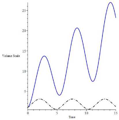
Рис. 1 ・ Evolution of volume scale V ( t ) for cases with (blue solid) and without (black dash-dot) Lyra geometry when spinor field nonlinearity simulates modified quintessence.

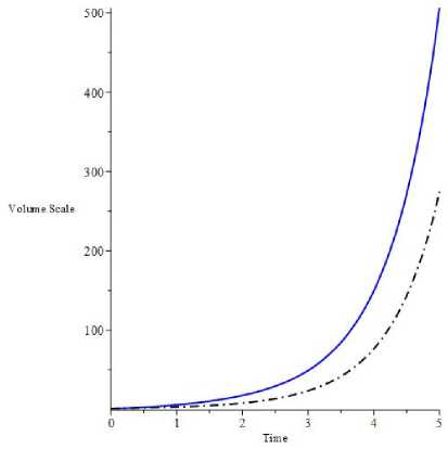
Рис. 2. Evolution of volume scale V ( t ) for cases with (blue solid) and without (black dash-dot) Lyra geometry when spinor field nonlinearity describes modified Chapligyn gas.

The foregoing system leads to three different cases:

• (i)    A ¹ = A ² = A 3 = 0. By virtue of Fierz identity in this case the spinor field becomes linear and massless;

• (ii)    A ² = A 3 = 0 and @ 2 = а з which gives rise to locally rotational symmetric Bianchi type-I (LRSBI) model;

• (iii)    @ i = @ 2 = @ з i.e. the anisotropy vanishes and BI spacetime becomes Friedmann-Lamaitre-Robertson-Walker (FLRW) one.

Thus if we consider the case (i) the R.H.S. of equation (26) becomes trivial nd in this case volume scame is a linear function of time, i.e.,

• V(t) = C o t + C i , C o , C i - consts.                               (32)

As far as other cases are concerned the results are similar to ones illustrated in figures 1 and 2. We plan to study these cases in details in some upcoming papers.

Concluding remarks

Within the scope of a Bianchi type-I cosmological model we have studied the role Lyra’s geometry if the universe is filled with spinor field. It is found the corresponding Einstein equations do not undergo any changes in forms which leads to the identical conclusions as in absence of Lyra’s geometry. Nevertheless, the invariants of spinor field depends on Lyra’s geometry, hence the final results differ from the ordinary one. Corresponding equations are solved numerically and the comparison of cases with and without Lyra’s geometry is displayed graphically. As in ordinary case, the nontrivial non-diagonal components of EMT of spinor field lead to three possibilities. In case of general BI model the spinor field becomes massless and linear. As a result the volume scale becomes a linear function of time. As far as two remaining possibilities are concerned, LRS BI model and FRW model we study in some upcoming papers.