Спорадические калиевые слои и их связь со спорадическими Е-слоями в области мезопаузы над Пекином (Китай )Sporadic

ions, as evidenced by the high temporal and spatial correlation between enhanced metal atoms and Es layers [Gardner et al., 1993; Friedman et al., 2000; Williams et al., 2007; Delgado et al., 2012; Dou et al., 2012]. However, no reports examined the relationship between the Ks and Es layers.

In this paper, using lidar and digital ionosonde observations from the newly launched Meridian Project, the aim of which is to help researchers better understand and predict space weather conditions over China, we statistically analyzed the Ks and Es layer events at Beijing. The observational data were obtained by the Na-K lidar at Beijing from November 2010 to October 2011 and from May 2013 to April 2014.

2.    DEVICES AND METHODS 2.1.    Na-K lidar

Our double-laser-beam lidar for K and Na layer measurements is an upgrade of the Beijing LIDAR used in the Chinese Meridian Project [Wang, 2010]. Figure 1 is the schematic of the lidar system. A twice secondary harmonic generation technique [Cheng et al., 2011] has been used. A pulsed Nd:YAG laser outputs a 1064 nm beam, which is sent into a frequency multiplier to produce a 532 nm laser beam. The remainder of the 1064 nm laser beam is sent into another frequency multiplier again, and thus we get two 532 nm laser beams. These

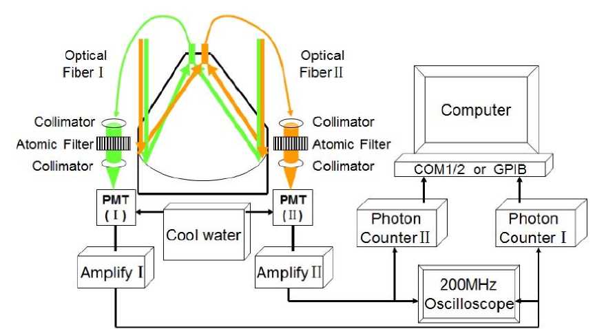
Collimator

Optical Fiber 1

Optical

Fiberll

Amplify I

Amplify II

Cool water

Photon

Counter I /

Computer

<"> Collimator llllllllllllll Atomic Filter

' Collimator [_COMjF2_ol_GP IВ

200MHz Oscilloscope

Photon

CounterII [..

PMT (П)

Collimator c 5

Atomic Filter (ШШШЕ1! !

PMT

Figure 1. Lidar system

two 532 nm laser beams are used to pump two dye lasers. A 589 nm laser beam is then produced to detect Na atoms, and a 770 nm laser beam is produced to detect K atoms. The repetition rate of the Nd:YAG laser is 30 Hz. The output energy of the 589 nm laser beam is 40 mJ per pulse, while for the 770 nm laser beam the output is 60 mJ. Backscattered fluorescence photons from the Na and K layers are detected by a Cassegrain telescope with a 100 cm diameter primary mirror.

Signals from 10000 laser pulses are integrated to produce a K layer profile (for a corresponding temporal resolution of 5.5 min); 5000 laser pulses are used for a Na profile (for a corresponding temporal resolution of 2.8 min). To increase the signal-to-noise ratio (SNR) in the K-layer data, a five point average in height is used in the analysis. The configuration of the lidar system is summarized in Table.

This Na-K lidar system was operated from November 2010 to October 2011 and from May 2013 to April 2014; about 2000 hr (209 nights) of data were collected with fairly good SNR (the background noise was generally no more than 250). The absolute densities of K atoms were obtained by using a standard inversion procedure and by considering the back-scattered cross section of K (D1) transitions, as well as the laser bandwidth.

The Ks layer events were selected according to the following criteria: (1) the maximum density of the Ks peak must be at least three times higher than that of the normal K layer at the same altitude (i.e., a strength fac-tor≥3); (2) the maximum density of the Ks peak must be more than 1/2 of the peak density of the normal K layer (because at high altitude, Ks events can be associated with a larger strength factor and a very low relative density); (3) the full-width-at-half-maximum (FWHM) of the Ks layer must be <3 km; and (4) the Ks event must last for at least three successive lidar profiles. These criteria are similar to those described by Gong et al. [2002].

Main Specifications of the Na-K Lidar System

	Na	K
Transmitter:
Wavelength, nm	589	770
Pulse energy, mJ	40	60
Line width, GHz	1.5	1.5
Pulse width, ns	~10	~10
Repetition rate, Hz	30	30
Beam divergence, mrad	<0.5	<0.5
Receiver telescope
Type	Cassegrain
Diameter, mm	~Ф1000	~Ф1000
Field of view, mrad	2	2
Receiver filter
Wavelength, nm	589	770
Bandwidth, nm	1	1

2.2.    Digital ionosonde equipment

Digital ionosonde equipment was also employed to study the correlation of sporadic Na s layer with sporadic E s layer. Our digital ionosonde which also belongs to the Meridian Project is located ∼ 24 km southeast of the lidar site in the Changping District (Beijing). In this configuration, the lidar and the ionosonde detect nearly a common volume in the mesopause region. The ionosonde records data automatically every 15 min, and its frequency scans from 0.5 to 15 MHz in 150 s to form a data file. For comparison, we chose data collected from November 2010 to October 2011 and from May 2013 to April 2014 at Beijing, which were obtained by both the ionosonde and the lidar. Reading the ionosonde SAO files makes the E_s-layer parameters available, such as its f o E s (the critical frequency) and h ^'E s (the virtual height).

3.    RESULTS

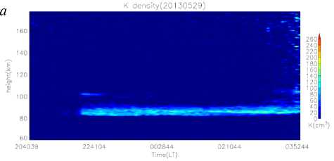
An example of the contour plot and the single profile at the moment when K s reached its maximum density at Beijing on May 29, 2013 are shown in Figure 2. As can be seen in Figure 2, a , the K s appeared at 22:18 LT and then disappeared at 22:43 LT. Thus, the duration of the K s event was about 1 h. From the profile at its maximum at 23:09 LT (Figure 2, b ), we can obtain its general properties. For example, the peak K density of K s is 161.25 cm^–3, the relevant altitude is 102.62 km, the FWHM is 0.29 km, and the strength factor is 6.83.

The seasonal distribution of K s occurrence at our location is shown in Figure 3, a . We noticed that the K s occurrence under study was not smoothly distributed over the year. As shown in the Figure, the K s occurrence has maximum value in January and July. The seasonal distribution of E s occurrence at our location is illustrated in Figure 3, b . Here, the digital ionosonde data are used for the analysis. We noticed that, unlike the K s events, the E s occurrence is smoothly distributed over the months of the year. The E s occurrence has maximum value in May, and the E s occurrence in the summer months is much higher than that in other seasons. In February, the E s occurrence is the lowest. From these observations it was evident that K s and E s occurrences are characterized by completely different seasonal variations.

The K s and E s events were also compared on a case-by-case basis. Owing to the limited number of ionosonde data, we could compare only 21 of the 58 K s events. We observed that 15 of the 21 events verified that K s events corresponded with E s events. A histogram comparing the time differences for the 15 pairs of events is given in Figure 4. In the previous study of Na s layers, researchers frequently compared the time of occurrence of Na s and E s layers to prove the mechanism

b

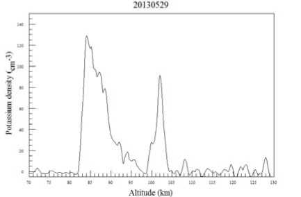
Figure 2. Contour of the K layer observed at the Beijing site from 20:40:39 LT on May 29, 2013 to 03:52:44 LT on May 30, 2013 ( a ); the K density profile observed at 23:16 LT ( b )

Figure 3. Seasonal distributions of K s occurrence (frequency and numbers) at our location and the observation time (days and hours) in each month ( a ); seasonal distribution of E s

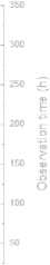
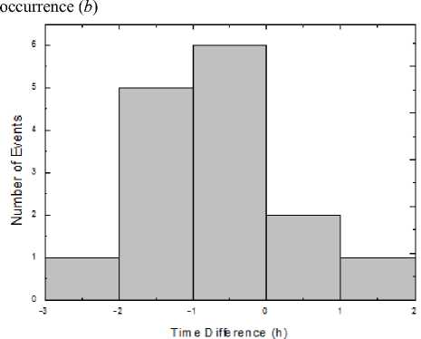
Figure 4. Distribution of the time difference between K s and E s (the negative value represents E s reaching its lowest height before K s reaches its maximum)

by which Na+ in the Es layer was neutralized to Na [Gong et al., 2002]. As deduced from the previous observation of the Nas layers, when Es descended to the lowest height with time, the Na density reached its maximum [Gong et al., 2002; Ma et al., 2014]. Therefore, we defined the time difference between Ks and Es in a similar way: the time difference refers to the time when a Ks event developed to its maximum intensity and an Es event to its minimum height, with the negative values representing Es reaching its minimum height before Ks reaches its maximum intensity. As shown in the Figure, all 15 associated Es events reached their minimum heights within 3 h before and 2 h after, with a mean value of less than 1 h before the corresponding Ks events reached their maximum intensities.

4.    DISCUSSION

The seasonal distribution of K s occurrence frequency is also quite different with that of E s . The maximum of E s occurrence frequency is observed in summer and the minimum in winter. These results are much different with those of K s , as many K s events were observed in winter. However, a relative good relationship between K s and E s was found in the case-by-case study. So we need to consider the most accepted mechanism by which metal ions are neutralized to form atoms in a descending E layer.

The height distribution of E s in different seasons is shown in Figure 5. The Y axis represents the lowest E s height in the observation night; the black circle marks different E s heights for different days, and the red line represents the fitted curve of the distribution. The distribution of E s heights presents a semiannual variation with minima in winter and summer, and the K s occurrence has two maxima in winter and summer, as seen from Figure 3, a . Due to the lower height of the winter E s , the K ion is more easily converted into K s , but the E s occurrence is lower in winter, because the E s layers have different contents of Na and K elements.

Neutralization of K⁺ occurs by forming a cluster ion with a ligand X, where X=N 2 , O 2 , O (in order of decreasing concentration in mesopause and lower thermosphere (MLT) region) [Eska et al., 1999]. The recombination is shown as follows:

K + +X(+M)—K + X (1)

K + X+Y—K + Y+X (2)

K+(XorY)+e-^K+XorY (3) where M is the third body (most likely N2 or O2). K+ is a relatively large singly-charged ion (cf. Na+). It forms very weakly bound clusters with the major species (N2, O2, and O) in MLT, with binding energies less than 20 kJ/mol. Therefore, the sequence of reactions (1)–(3) becomes significant at very low temperatures characteristic of summertime MLT [Plane et al., 2014].

Ernest Kopp pointed out that Na ions in the ionosphere are about ten times of K ions [Kopp, 1997]. Although Na ions are about a few hundreds, it is difficult to produce Na s . Although the K ion density is only about a few dozen per cubic centimeter, K density is also only about a few dozen per cubic centimeter, so that K ions are more prone to produce K s . So, compared to other months, the E s layer contains more K ions in January. Furthermore, it is easier to produce K s events through ion–neutral reactions.

5.    CONCLUSION

Of two years of lidar observations, 58 K s events are observed in 2000 hr of data. Seasonal distributions of K s occurrence were obtained, with two maxima found in July and January. Many K s events occurred in November, January, and February (especially in January).

The relation between K_s and E_s was analyzed. The K s and E s occurrences have different seasonal variations. The K_s occurrence has a maximum in July and a secondary maximum in January, but the E s occurrence has a minimum value in winter. The probable reason for the high occurrence of K s in January is that it is easier to produce K s events through ion–neutral reactions, considering that the E_s layer contains relatively more K ions in January. However, the relatively good relation between K s and E s was found in the case-by-case study. The K ion is more easily converted into K s because E s heights are relatively low in winter. So, we need to consider the most accepted mechanism by which that metal ions are neutralized to form atoms in the descending E

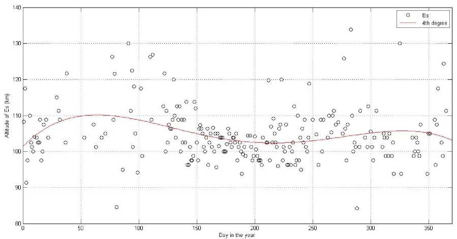
Figure 5. Height distribution of E s events in the year. The black circle represents different E s heights for different days; the red line marks the fitted curve of the distribution

layer. As a consequence, more combined observations are needed to develop further understanding of the K s formation mechanism.

We acknowledge the use of the data from the Chinese Meridian Project . The work was supported by the Natural Science foundation of China (the grants No. 41474130, 41264006), NSSC research fund for key development directions, the Specialized Research Fund for State Key Laboratories of China, and China-Brazil Joint Laboratory for Space Weather, CAS.