Stability of solutions to the stochastic Oskolkov equation and stabilization

The Oskolkov equation

( I - x A)A u = v A ² u - ^d(^ul                  (1)

d ( x i ,X 2 )

describes the plane-parallel flow of a viscoelastic liquid [1]. In [2], the initial boundary value problem for the equation in D x R was studied, where D C R 2 x 1 _x 2 ) is a region with a smooth boundary. The smoothness and simplicity of the set, which is a phase space, is proved. In [3] studied the stability of solutions to equation (1).

We extend the results of [3] to the stochastic equation (1). To do this, we consider equation (1) as a stochastic semi-linear equation of the Sobolev type

Ln = Mn + N ( n ) ,                             (2)

o where, П is the Nelson — Gliklikh derivative [4] of the stochastic process n = n(t)- The number of works on the study of stochastic equations of the Sobolev type is constantly growing. For example, in [5–7] study the solvability of a linear equation

L n = Mn.(3)

The papers [8, 9] consider the stochastic phase space of a nonlinear equation

L°n = M (n).(4)

The article [10] considers the stability of the stochastic linear Oskolkov equation

(I — xA)Aut = v A2u.

Equation (5) is considered a linear stochastic equation (3). In the papers [11–13] find numerical stable and unstable solutions to equation (3). In the papers [14, 15] study the invariant manifolds of equation (2). The stabilization problem for equation (3) was considered and solved for the first time [16].

This article is a continuation of the work of [10] on the stability of the semilinear equation (1). Before proceeding to the study of the stability and instability of solutions to the stochastic Oskolkov equation, it is necessary to address the solvability of the stochastic equation (1). To do this, we extend the results of [1] to the stochastic Oskolkov equation. Then we apply the results of [15] to prove the existence of invariant spaces of the stochastic Oskolkov equation. To solve the problem of stabilizing unstable solutions to this equation, we extend the results of [16] to the semilinear equation (2).

The article contains three parts. The first part presents the results of the stable and unstable invariant manifolds of equation (2). The second part is devoted to the stabilization problem. In the third part, the results of the first and second parts are applied to the semilinear stochastic Oskolkov equation.

1.    Invariant Manifolds of Stochastic Sobolev Type Equations

Let the space U (F) be a separable Hilbert space, {vk} ({^k}) is the basis of the space U (F), {Ck} ({Zk}) is a sequence of random variables from L2, and K = {Ak C R+} is a ∞ sequence of real numbers, ^ A2k < to. The space UKL2 (FKL2) is a replenishment of the k=1

linear shell of random variables of the form

∞∞ n = $2 AkCk Vk I z = 52 Ak Zk ^k I k=1               k=1

according to the norm

ІІФІіи,

K L 2

∞

= EAkDCk •  ІК »FkL2 = k=1          \

∞

E AkDZk • k=1       /

Lemma 1.

The

operator A G    L( U ; F )    iff the same operator

A ^{G L (U} K L 2 ; F K L 2 ) .

Let operators L, M G L( U _K L ₂ ; F _K L ₂ ), N G C “ ( U _K L ₂ , F _K L ₂ )• Consider a semilinear stochastic equation of the Sobolev type (2) with an initial condition

∞

n(0) = 52 A k C k V k • k =1

Stochastic K -process n G C ¹ (J; U K L ₂ ) we call the solution of equation (2) if probably almost all its trajectories satisfy equation (2) for all t G J , where J C R . The solution of П = n(t) of equation (2) is called the solution of the Cauchy problem (2), (6) if the equality (6) holds for some random L -value n o G U _l L ₂ •

Definition 1. [8] The set P C U _L L ₂ called a stochastic phase space of equation (2) if

• (i)    probably almost every solution path n = n(t) of the equation (2) lies in P ;

МАТЕМАТИЧЕСКОЕ МОДЕЛИРОВАНИЕ

• (ii)    for almost all n _o G P exists a solution to the problem (2), (6).

If the operator M ( L,p )-bounded operator, then operators

P = — [(LL - M ) ^{- 1} Ldp, Q = — / LUL - M ) ^{- 1} dp 2пі                          2ni

γ

γ

are projectors, where the contour ү bounds o ^L (M ). Denote U K L 2 = im P . The subspace U K L 2 is the phase space of equation (3) [5].

Theorem 1. Let the operator M (L,p)-bounded operator, operator N G C 1(UkL2, FKL2), and the set f {П G UkL2 :(I - Q)(Mn + N(n)) = 0}, if ker L = {0}; I UkL2, if ker L = {0} is a simple Banach C^manifold. Then the set M is the phase space of equation (2).

The proof of the theorem repeats the proof of a similar theorem in [8]. Therefore, it is not given here.

Let the following condition be fulfilled:

o ^L (M ) = of (M ) u^L (M ) ,           1

o^ l ) (M ) = {p G o ^L (M ) : Re ^ >  0 (Re ^ >  0)} у

There are projectors

P i ( r ) 2 / ^L - M) ^{- 1} LdL

^Y l(r)

Denote I ^s = im P l and I ^u = im P r . If operator M ( L,p )-bounded operator, then the spaces I ^s and I ^u are stable and unstable invariant spaces of equation (3) [10].

Consider the set

M s = ^{n o ^G U K L 2 ^: ||P l n o || u _K L ₂ <  R I , ||n ^{( t,} n o ⁾ ^ U _L L ₂ ^ R 2 , t ^{G R} + ^}

^ M u = ^{n o ^G U K L 2 ^: ^P r n o ||u_k L ₂ <  R I , ^|n ^{( t} , n o ^{) |} U L L ₂ <  R 2 , t ^{G R} - ^})-

If the set M ^s ( M ^u ) is diffeomorphic to a closed ball in I ^s ( I ^u ), touches I ^s ( I ^u ) at the zero point, and | n ( t, n _o ) I U _L L ₂ ^ 0 for any n _o G M s ( n _o G M u ) and for t ^ +ro ( t ^ —x), then the set M ^s ( M ^u ) is called the stable(unstable) invariant manifold of equation (2).

Theorem 2. [15] Let the operator M (L,p)-bounded operator, condition (7), and the operator N G C k ( U, F ) , N (0) =0 , N' _o = O . Then there are stable and unstable invariant manifolds of equation (2) in the neighborhood of the point zero.

2.    The Stabilization Problem

For stabilizing solutions, it is required to find such a control effect on equation (2) so that its solution n = n ( t ) becomes stable, i.e.

,lim ІШІІи^ =0 tx+^

Let condition (7) be fulfilled, then equation (2) will be considered as a reduced system

Lo П= Mon0 + No(n0 + ns + nu),(9)

Ls ns = Ms ns + Ns (n° + ns + nu),(10)

Lu Пи = Munu + Nu(n0 + ns + nu),(11)

where F _o ( n ⁰ + n s + n u ) = ( I - Q)N ( n ⁰ + n s + n u )■ The initial condition (6) is split as follows:

По = (I - Q)n0 =              ^k^k^k, k={k:ker L={0}} ns = Pl РПО = Pl ПО =     52     ^k^k ^k ’ k={k:^k EaL (M)} nU = Pr Pno = Pr По =     52    ^k ^k ^k • k={k:^k EaL (M)}

If the stochastic process n = n(t) is the solution of equation (2), then this process satisfies system (9) – (11). Moreover, the solution of system (9) – (11) can be written as:

n = n^0(t) + n ^{s (t)} + n ^{u (t)},                                 ⁽¹²⁾

where n ⁰ = n ⁰ ( t ) is the solution of equation (9), n ^s = n ^s ( t ) is the solution of equation (10), n ^s = n ^u ( t ) is the solution of equation (11).

Consider the following stabilization problem . Let us find such a stochastic process χ that condition (8) is satisfied for the solution of the system

О

Lo n°= Mon° + No(n° + ns + nu),(13)

Ls ns = Ms ns + Ns (n° + ns + nu),(14)

О

Lu nu= Munu + Nu (n° + ns + nu) + X.(15)

Part of the relative spectrum of a^La (M s ) lies in the left half-plane of the complex plane. From theorem 2 it follows that

. lim llns(t)^UKL2 =0.

t ^+ж

The stochastic process of χ is determined using feedback

X = Bnu.(17)

Let us find an operator B such that the spectrum a ^Lu (M u + B) lies in the left halfplane of the complex plane. Denote m = max {Re ^ : Re ^ >  0}. Let operator B have ^^Ea L ^{( M} )

the form

B = -( _{e +} m ) I,                                (18)

МАТЕМАТИЧЕСКОЕ МОДЕЛИРОВАНИЕ where е > 0 can be arbitrarily small. Then the relative spectrum aLu (Mu + B) lies to the left of the imaginary axis. From theorem 2 it follows that

lim ||nu( t)|| u _K L 2 = ⁰ - t→ + ∞

The solution n = n(t) of system (13) — (15) can be written as n = (I + 6)(n1) = (I + 6)(ns + nu), where the diffeomorphism 6 = P-1. Then, for system (13)-(15) with feedback(17), by virtue of equalities (16) and (19), equality (8) will be fulfilled.

3.    Invariant Manifolds of the Stochastic Oskolkov Equation

Let

U = {u G W 4 : u(x 1 ,x ₂ ) = Au(x 1 ,x ₂ ) = 0 , (x 1 ,x ₂ ) 6 d Q} , F = L 2 ( D ) .

The basis in space U ( F ) is a family of eigenfunctions {^ k } of the Laplace operator A, orthonormal with respect to the scalar product (•, •) ([• , •]) in U ( F ). Define the operators

d ( n, An) d ( x i ,X 2 ) .

L : n ^ ( A — A)A n, M : n ^ v A 2 n, N : n ^

Operators L, M G L ( U k L 2 , F k L 2 ).

Lemma 2. (i) The operator M is (L, 0)-bounded;

(ii) the operator N G C “ ( U K L 2 , F K L 2 ) , N (0) = 0 , N 0 = O .

Proof. (i) The relative spectrum of the operator M has the form

Sw ) = I

νν k

1 — XV k

: k G N \{l : X 1 = v i }^j ,

and is obviously limited. Here {vk} is the spectrum of the operator A. Then the operator M (L, a)-bounded. The kernel of operator L has the form ker L = ! {0}, X 1 = Vk’ k G N; { Wk}, X 1 = vk.

Let ф G ker L \{0}, i.e.

v =         a i ^v i , 52 | a i | > ⁰ ,

χ-1=νl       χ-1=νl then ф G ker L \ {0}, v = 52 aiфі, 52 |ai| >0, χ-1=νl       χ-1=νl and

MV = vx ^{- 1} 52 a k V k / imL. χ ^-1 = ν k

• (ii)    Let us calculate the Frechet derivatives

d ( n, A-) _ d (• , A n) , N ‘‘ =   d (• , A-) _ d (• , A-) d ( x i ,X 2 ) d ( X 1 ,X 2 ) , ⁿ       d(x i ,X 2 ) d ( x i ,X 2 )

All other derivatives are zero. Note, that N '_n , N E L( U K L 2 , F K L 2 ), and N (0) = 0, N 0 = O.

□

Consider the set M and the space U ¹ _K L 2 . They have the following form:

\ U K ^L 2 ^{, x 1} / ^{v k ^} ;

1 {n E UkL2 : (Mn + N(n), Vi) = 0, X-1 = vi}, i          UKL2, x 1 / {vk};

U K L ²    t { n E U k L 2 : fan) = 0 , X - ¹ = v i} •

Theorem 3. Let A E R, v E R \ {0} . Then the set M

• (i)    is a simple Banach C ^∞ -manifold;

• (ii)    is the phase space of stochastic equation (1) .

Let v > 0, then a(M)L = a(M)L U a(M)L, where aL(M) = I 1 vvk   : vk > X—1! , aL (M) = I  vvk   : vk < X-1] •

• 1    — Xv k                         1 — Xv k

Consider the spaces

I ^u = {n E U k L 2 : (n, V k )V k = 0 , v k >  x 1 } ,

I ^s = {n E U k L 2 : (n, V k )V k = 0 , v k <  x^{- 1} }, and consider the invariant sets

M u = {n E M : n = $2 A k ^Vk } , M s = {n E M : n = 52 A k ( k V k } • k : ν k >χ ^-1                                             k : ν k <χ ^-1

Theorem 4. Let x E R - , v E R ₊ . Then the set M u is a finite-dimensional unstable invariant manifold of stochastic equation (1) , and the set M ^s is an infinite-dimensional stable invariant manifold of stochastic equation (1) .

aL u (Mu + B ) = [E—E^El I

1 _ Xvk lies in the left half-plane of the complex plane.

Let the parameters x = _0 , 1, v = 0 , 1. Fig. 1 shows a graph of the solution of the stochastic Oskolkov equation before stabilization, and Fig. 2 shows a graph of the solution after stabilization for ( 1 = 0 , 2353939952, ( 2 = _1 , 079196234, ( 3 = -0, 1231141571, ( 4 = 1 , 625165927 in section x ₂ = 1.

МАТЕМАТИЧЕСКОЕ МОДЕЛИРОВАНИЕ

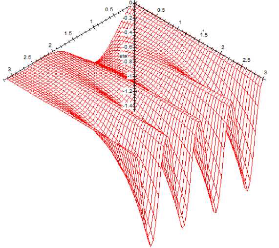
Fig. 1 . Graph of the solution of the stochastic equation (1) before stabilization for x = -0 , 1, v = 0 , 1

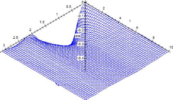
Fig. 2 . Graph of the solution of the stochastic equation (1) after stabilization for x = —0 , 1, v = 0 , 1

Conclusion

In the future, we propose studying the stability of equations of form (2) in a relatively sectorial case. We also propose finding a method for solving the stabilization problem in the case when the relative spectrum intersects with the imaginary axis.