Structural Conditions on Observability of Nonlinear Systems

Published Online August 2011 in MECS

During the analysis of process, a basic question is that whether the system states are uniquely determined by output data. Especially, for a given dynamic description and observation of a system, we need to know the conditions by which the initial states are uniquely determined by output data in a given time interval. This is observability. For observability, it is a property of systems, which is determined by two aspects: the differential equations and outputs [1].

Hwang and Seinfeld [2] investigated the observability of nonlinear systems and got the sufficient and necessary conditions of observability. They extended the sufficient and necessary conditions of observability in linear time varying systems to the nonlinear systems with linearized states form. It can be determined the local observability with any initial conditions and calculated for the whole initial domain. Hermann and Kerner[3] summarized the controllability of nonlinear systems and gave the conceptions of observability of nonlinear systems. These conceptions were defined with the method as that of controllability. The observability rank condition and observability criterion were given by using Lie algebra. Knobloch[1] explored a class of autonomous nonlinear system. The observability criterion was obtained by evaluation of “approximation first integrals”. This concept is borrowed from nonlinear control theory where

Footnotes: 8-point Times New Roman font;

Manuscript received January 1, 2008; revised June 1, 2008; accepted July 1, 2008.

Copyright credit, project number, corresponding author, etc.

it appears under the label “Dissipation Inequality”. Bartosiewicz[4] researched the local observability of nonlinear systems. The sufficient and necessary conditions of analytical systems were obtained. These conditons are expressed with the language of ideals of germs of analytic or smooth functions and real radicals of such ideals.

In the presented paper, parameter space is introduced to the analysis of nonlinear systems and used to research the observability. Lu etc [5-8, 11] studied the linear systems and electrical networks with parameter space conception first. Some structural observability conditions for linear systems were obtained and applied to analyze linear systems over the field of F ( z ). The obtained conditions in this paper are called structural observability conditions of nonlinear systems, because parameter vector is contained in this observability condition, i.e., these conditions can show the effects of parameters to systems observability. Parameters taking values in parameter space maybe change the observability of the system, so measurement conception is introduced and shows that if the system is structural observable then the measurement of points set which make the system is not observable is zero.

The rest of this paper is organized as follow: in section 2 the structural observability rank condition and distinguishability are given; in section 3 the structural observability condition and unidentifiability of solutions are given based on differential geometry; in section 4 we research the structural observability problem by algebraic method; in section 5 examples are used to illustrate the application of condition.

• II.    STRUCTURAL OBSERVABILITY RANK CONDITION AND DISTINGUISHABILITY

In this section the conception of structural observability rank condition for nonlinear systems is presented, which is important to obtain the structural observability criterion. The way to obtain the structural observability condition is similar to that in [3]. The relationship between observability and distinguishability is discussed also.

• A.    Structural Observability Rank Condition

where u e U , U is a subset of R l , x e M , M is the connected smooth manifold with dimension n . У e R m , f and h are smooth functions, z = ( z _i, L , z q ) e R q is a parameter vector with dimension q of the system, R^q is called the parameter space.

The set of all smooth vector field on M is a infinite dimension real vector space, denoted by X ( M ) . Lie algebra is denoted by the multiplication of Jacobi bracket [ g ₁, g ₂ ] as follow:

• [ g i , g 2 ] — ⁽ x ) g i ⁽ x ) — ⁽ x ) g 2 ⁽ x ) ⁽²⁾ оx оx

where g 1 , g ₂ and [ g 1 , g ₂] e X ( M ), then the member of X ( M ) is denoted to column n -vector valued functions of x . For any fixed g 1 e X ( M ), a real linear transformation from X ( M ) to itself is a map with the form g ₂ ^ [ g 1 , g ₂ ], and is called Lie derivative respect to g 1 , denoted by L .

g ₁

Let C ” ( M ) denote the infinite real vector space consisted of all smooth real functions on M . X ( M ) can be acted as a linear operator on C ” ( M ) by the definition of Lie derivative. If g e X ( M ) , фЕ C ” ( M ) , then L_g ( ф ) e C ” ( M ), denoted by

L ⁽ ф ⁾⁽ x ) ^- ^ф x ) g ⁽ x ) g d x

For nonlinear system (1), we denote by H ⁰ the subset of C ” ( M ) containing h _i,L , h m , and by F 0 the subset of C ” ( M ) containing f i ,L, f n . Let H denote the smallest linear subspace of C ” ( M ) containing H 0 which is closed with respect to Lie derivative by elements of F ⁰ . (it should be note that f_i , h_j are functions with parameter z , i = i,L n , j = i,L , m ). A member of H is a finite linear combination of functions of the form:

L_f 1 _{( z )}(L L_f k _{( z )}( h i ( z ))L) (3) where f j ( z ) = f ( x , u j , z ) is a vector field with some constant u j e U .

Clearly, if g _i( z ), g ₂( z ) e X ( M ) and ф ( z ) e C ” ( M ) then

L , ,( L ₍M z )) - L , ,( L , ф( z )) = L ф( z ) (4) g i ( z )^v g 2 ^{( z ) ф} 77 g 2 ^{( z} )^V g i ^{( z ) ф 77 [} g 1 . g 2 Г ^ф 7X7

Let X ¹ ( M ) denote the linear space of all 1-form on M , that is, the finite combination of gradient of elements on C ” ( M ). We can define a subset of X ⁱ( M ), denoted by dH 0 = { dф: фe H 0 } and a subspace denoted by dH = { dф : ф e H } . Just as vector fields act on functions and other vector fields by Lie derivative, they act on 1-forms by the definition as follow:

Lg(w)(x) = gT(x) ^w-(^ ) + w(x) |g(x) (5) dx оx where w e Xi (M), g e X(M) . If w = dф , then Lg and d can exchange as:

^L _g ^{( d} ф ⁾ = d ^{( L} _gф ⁾

From the above, we can see that dH is the smallest linear space of 1-form containing dH ⁰ . The element of dH is the finite linear combination with the form: d ( L f i ( z ) (L L_f k ( z ) ( g i ( z ))L)) = L f i ( z ) (L L_f k ( z ) ( dg,( z ))L)(6) also where f j ( z ) = f ( x , u j , z ) is a vector field with some constant u _j e U .

Definition 2.1 : Nonlinear system (1) is said to satisfy the structural observability rank condition at x ⁰ ( z ) , if dim dH ( x ⁰ ( z )) = n ; if for any x ( z ) e M , dim dH ( x ( z )) = n holds, then systems (i) is said to satisfy the structural observability rank condition.

Remark 2.1 : For there contains parameter vector z in Definition 2.1, this rank condition is said to be structural observability rank condition, which show the effects of parameter vector z to this condition, i.e., parameter vector z taking values in parameter space maybe lead to dim dH ( x ( z )) <  n . All the parameter vector z such that dim dH ( x ( z )) <  n may form a set denoted by S , but for a nonlinear system who satisfy the structural observability rank condition the Lebesgue measurement of set S is zero, which is the meaning of term “structure”.

• B.    Observability and Distinguishability

We know that we can define the observability of systems by the definition of distinguishability.

Definition 2.2 : Given two system states x ₁ and x ₂ , we call them indistinguishable, denoted by x ₁ Ix ₂ , if there exists a input u ( t ) , t e [ 1 ₀, t _i] such that y ( x _i( u ( t ))) = y ⁽ x 2 ⁽ u ⁽ t ))) .

Definition 2.3 : Let { g } denote a set and s * { g } denote the Lebesgue measurement. For any z e R q , if the Lebesgue measurement of a set whose elements make nonlinear system (1) indistinguishable is zero, then this system is said to be structural distinguishable.

Definition 2.4 : Nonlinear system (1) is said to be structurally observable at x ⁰( z ), if I ( x ⁰( z )) = { x ⁰( z ) } ; if for arbitrary x ( z ) e M , I ( x ( z )) = { x ( z ) } holds then the system is said to be structurally observable.

Definition 2.5 : Nonlinear system (1) is said to be structurally weak observable at x ⁰ ( z ) , if there exist a neighborhood of x ⁰( z ) such that I ( x ⁰( z )) = { x ⁰( z ) } I D ; if for arbitrary x ( z ) e M , I ( x ( z )) I D = { x ( z ) } holds then the system is said to be structurally weak observable.

Ш . STRUCTURAL OBSERVABILITY CONDITION OF

NONLINEAR SYSTEM

In this section the structural observability condition of nonlinear system (1) will be presented after a Lemma is introduced first which is important to prove the condition.

Lemma 3.1 : Let V be a open subset of M , if x 0 ( z ), x ¹ ( z ) e V and x 0 ( z ) Ix ¹ ( z ) , then for arbitrary ф(x ( z )) e H , ф(x 0 ( z )) = ф(x ¹ ( z )) holds.

Proof: If x0 (z)Ix1 (z) , then for arbitrary k > 0 , any piecewise constant uj e U , small time sj , j = 1,L , k and output function hi, i = 1,L , m , by Definition 2.2 we have

h ( r k oLo r 2 o r ¹ ( x ⁰ ( z ))) = h ( r k oLo r 2 o r ¹ ( x ¹ ( z ))) (7) s_k s ₂ s ₁ s_k s ₂ s ₁

where rsk denotes the flow of fk (x) = f (x, uk, z) . Then we get the derivative respect to the times sk ,L, s2 ,s1 in equation (7) in turn, and because dhi _ d h drsk - d h fk = T , ,      ~ к j           f     Lfkhi ds,   dr   ds,    dr          1

sksk

Then

L_f 1 ₍ z ) (L L f k ₍ z ) ( h )L)( x ⁰( z )) = L f 1 ₍ z ) (L f ₍ z ) ( h i )L)( x 1 ( z ))

i.e., H is spanned by the form Lf1(z) (L Lfk(z) (hi(z))L) , so ф(x0 (z)) = ф(x1 (z)) .

Theorem 3.1 : If nonlinear system (1) satisfy the structural observability rank condition at x ⁰ ( z ) , then the system is locally structural weak observable at x ⁰ ( z ) .

Proof : For the system (1) satisfy the structural observability condition at x ⁰ ( z ) , i.e., dim dH ( x ⁰ ( z ))

= n , there exists n functions ф ₁,L , ф_п e H such that dф₁,L , dф_n are linear independent. Then we can define a mapping as follow:

x ^Ф( x ) = ( Ф 1 ,L, ф_п ) (10) Then d Ф is nonsingular at x ⁰( z ). So Ф is a one-to-one mapping in the neighborhood D of x ⁰ ( z ). Let V c D is a open neighborhood of x ⁰ ( z ) , then according to Lemma 3.1 we know that there exist no x 1 ( z ) e V such that x ⁰ ( z ) I_V x ¹ ( z ) for Ф is a one-to-one mapping. So I_Vx ⁰( z ) = { x ⁰( z ) } , i.e., system (1) is locally structural weak observable at x ⁰ ( z ) .

Remark 3.1 : Parameter z taking values in parameter space R^q does not change the distinguishability of the same state with different parameter z if system is structural observable. If two parameter p 1 , p ₂ e R q are indistinguishable then we can have the following Theorem.

Theorem 3.2: For two parameters p1, p2 e Rq , if p1IV p2 and p1 such that system (1) satisfy the observability rank condition at x(p1 ) , then there exist a neighborhood Vp2 of x(p2) and a mapping X: Vp2 ^ Vpi such that X(x(p2)) = x(p1).

Proof: Since p1 IVp2 , the output y = h(x, z) of (1) satisfy yp = h (S p1) = h (S p 2) = yp2

• i .e., h i ⁽g, p 1 ) = h i ⁽g, p 2 ), ^then

Lf 1 ( z ) (L ^Lf^k ( z ) ⁽ h i ) ^L ) = Lf 1 ( z ) (L L k ( z ) ⁽ h i ) ^L ) .

For a neighborhood W of x ( p ₁ ) , we have

Hp2(x(p2)) = Hp1(x(p1)) e HP1(W), then for the neighborhood Vp2 of x(p2 ) , Hp (V ) c Hp (W) holds. Take X : Vp ^ Hp' (Hp (x)), p2 p2            p1                                          p2           p1 p2

then for state x ( p ₂) there exist a transformation X such that X ( x ( p ₂)) = x ( p 1 ).

Remark 3.2 : For system (1), since the nondistinguishability of parameters p ₁ , p ₂ e R^q , then there exists a transformation between the solutions x ( p ₁ ) and x ( p ₂ ) with same time but different parameters such that X ( x ( p ₂)) = x ( p 1 ) . At the same time, the nondistinguishability of parameters leads to the nonobservability of systems.

^ . ALGEBRAIC CRITERION ON STRUCTURAL

OBSERVABILITY CONDITION OF NONLINEAR SYSTEMS

In section Ш we discuss the structural condition on observability of nonlinear systems from the view point of differential geometry. Here we will consider the observability problem based on algebra. Some basic notations and terminologies we refer readers to reference [12].

Definition 4.1 : The element of quotient field K of the ring of analytic functions is called meromorphic function.

Here we just consider the so-called input affine nonlinear system, that is, in system (1) the state equation can be described as the combination of input u and another function in state x, which is of the form as follows:

j& = f ( x , z ) + g ( x , z ) u y = h ( x , z )

where state x e R n , input u e R m and output y e R^p . The elements of function vectors f and g are meromorphic functions. The notation z is also the parameter vector, which has q dimension and belongs to parameter space R^q .

Now we can define three spaces X, Y and U respectively, which denote X= spanK {dx} , U= spanK {duj, j > 0} and Y = U i>0 Y(i), where Y(i) = spanK {dyj, 0 < j < i}. The subscript K denotes the field of meromorphic function, that is, all the elements of these three spaces are meromorphic functions. Then a sequence of subspace is obtained as follows:

0 c O ₀ с O 1 с O 2... с O k с ...         (12)

where the notation O _k @ X I ( Y ⁽ k ) + U ) is said to be the observability filtration.

Naturally, we take the limit of observability filtration to infinite, which can be denoted as O∞, then easily we get

O „ @ X I ( Y + U )           (13)

We take a linear system as an example to show how to get the k-th observability filtration Ok. Given a linear system as follows:

x = Ax + Bu y = Cx

According to the construction of space Y(i), we continue step to step to get Ok:

First step: dy = Cdx ;

Second step: dy = CAdx + CBdu ;

Third step: dy ⁽²⁾ = CA ² dx + CABdu + CBdUk

M

Since X =span _K { dx } , then by k step we get

O _k = span K { Cdx , CAdx ,L , CA k dx }

Remark 4.1: For system (11), we know that it contains the parameter vector z, all the spaces X, Y and U and subspaces Ok and O∞ are spaces in parameter vector z. It is very important to notice parameter vector z in these spaces, because the parameter vector z may change the property of these spaces, which we are interested in.

Definition 4.2 : The subspace O ∞ is called the structural observability space of nonlinear system (11).

We will first give a Lemma before giving the algebraic criterion on structural observability of nonlinear system (11). This Lemma can describe a property of structural observability space O ∞ .

Lemma 4.1 : The structural observability space O ∞ of nonlinear system (11) satisfies the following equality:

• 1-    _n      ._r d( y , y L, y ⁽ n ^-1))

dim O ∞ = rank[              ]

d x

Proof: According to the construction of structural observability space O∞, we know that dimO∞ = min (dim X, dim (Y + U)). Of course the dimension of X is n, because space X is spanned by the differential of n states. Since Y = U i>0 Y(i) and Y(i)=spanK {dy1,0 < j < i}, space Y can be denoted as Y= spanK {dy1,0 < j}, that is, any dy* and dy1 are independent with each other, i, j > 0 , i ^ j . If dim(Y + U) > n, the dimO2 =dimX= n. If dim(Y + U) < n, for example k, then the dimO∞ = dim(Y + U) = k. Now we chose the first n elements from space Y, that is, dy* , i = 0,1,2,L , n -1 , and we know the n elements are independent with each other. So we differentiate them with respect state x with the form

d( y, yL, y(n-1)) dx        ’ it is clearly that the Jacobin matrix has the full column rank n. so the maximum dimension of structural observability space O∞ is n. If we chose the first k (< n) elements from space Y, the dimension of structural observability space O∞ is equal to number of elements chosen from space Y.

Thus we complete the proof.

According to Lemma 4.1, we know the structural observability space O ∞ has some relation to space Y . Following we will give the structural observable algebraic criterion.

Theorem 4.1 : Nonlinear system (11) is said to be structural observable if and only if O ∞ = X .

Proof : For sufficiency: we know O „ @ X I ( Y + U ) = X , then we can chose first n elements from Y , that is, dy* ( i = 0,1,2,L, n - 1). According to Lemma 4.1 it is known that the Jacobin matrix

d( y, yL, y(n-1)) dx has full column rank n. then we can say that the state x of nonlinear system (11) is determined by output data y and its differentials only, which is the meaning of structural observable.

For necessity: since nonlinear system (11) is structural observable, then its output has (n-1)-order differential, dyi ( i = 0,1, 2,L, n - 1 ) and any two different dyi are independent with each other. Then by Lemma 4.1 it is known that dimO∞ =dimX= n and O∞=X holds.

Here we complete the Theorem.

From Lemma 4.1 and Theorem 4.1 immediately we get the following Theorem.

Theorem 4.2 : Nonlinear system (11) is said to be structural observable if and only if

d( y, yL, y(n-1))_ rank[                ] = n dx

Proof : According to Lemma 4.1 and Theorem 4.1 the proof of Theorem 4.2 is obviously.

V . APPLICATIONS

In this section, we will use several examples to show the applications of structural observability condition.

Example 5.1 : First we consider a linear system with the form as follow:

;& = A ( z ) x + B ( z ) u y = C ( z ) x

where, A ( z ) , B ( z ) and C ( z ) are matrices in parameter z with proper dimensions as that in system (1). Clearly, F 0 = { A(z ) x + B ( z ) u , u e U } . So the Lie algebra generated by F ⁰ is { A(z ) x , b i (z ), i = 1,L , l } , where b_i ( z ) is the i -th column of B ( z ) . By calculation it is known that the smallest subalgebra containing F ⁰ is spanned by

{ A ( z ) x , A j ( z ) b i ( z ), i = 1,L, l , j = 0,1,L , n - 1 } .

Let c_k ( z ) denote the k -th row of C ( z ) , then for r > 0, p > 0 , we have

L A ( z ) x c k ⁽ z ) ^Ar ⁽ z ) x = c k ⁽ z ) ^Ar ⁺ 1 ⁽ z ) x

L A ' ( z ) _M z ) C k ( z ) A ^P ( z ) x = C k ( z ) A r ^{+ P} ( z ) b ( z )

L A ( z ) x c k ⁽ z ) ^{A P (} z ) ^bi ⁽ z ) = L A - ( z ) b i ( z ) c k ⁽ z ) ^{A P (} z ) ^bi ⁽ z ) = ⁰

So by Cayley-Hamilton Theorem it is known that H is spanned by

{ck(z)Ar(z)x, ck(z)Ar(z)bi(z), k = 1,L , m, i = 1,L, l, r = 0,1,L , n -1}, then dH(x(z)) is spanned by

{ c_k ( z ) A r ( z ), k = 1,L, m , r = 0,1,L , n -1 } .

So dH ( x ( z )) has the constant dimension. If the dimension of dH ( x ( z )) is n , then by Theorem 3.1 the linear system (15) is structural observable (we should notice that for linear system there is no difference between local observability and global observability).

We continue to consider this example from the view point of algebra. For linear system the structural observability condition can be changed to the well known rank condition. From section IV it is known that for linear system (14), the k -th observability filtration O k = span K {Cdx , CAdx ,L , CA k dx } . Then we just need to ensure that whether the space of O n -1 is equal to space X . For linear system (15), structural observability space O n -1 = span K { C ( z ) dx , C ( z ) A ( z ) dx ,L , C ( z ) A ( z ) ” ^{- 1} dx } . So if the rank of matrix [ C ( z ), C ( z ) A ( z ),L , C ( z ) A ( z ) ” ^{- 1}] ^T is n , we can say that the basis spanning space O n -1 is transformed by basis of space X , so space O n -1 and X are same, that is, by Theorem 4.1 O ∞ = X holds which implies the linear system (15) is structural observable. Using Theorem 4.2 we can get the similar calculation and the same conclusion that linear system (15) is structural observable.

According to [5,6], if we want to justify whether a linear system over F(z) such as system (15) we can calculate whether rank (T o ( z )) = n is true or not, where T o ( z ) = [ C ( z ), C ( z ) A ( z ),L, C ( z ) A ( z ) " ^{- 1}] ^T is called the observability matrix of this linear system. Linear system is structural observable iff det( T_o^T ( z)T_o ( z )) ^ 0 .

Example 5.2 : We still consider a linear network shown by Fig. 5.1. It is a multi-input multi-output system containing two sub-networks.

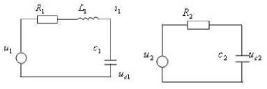
Fig. 5.1 Network structure

The system has five physical parameters R ₁ , L ₁ , C ₁ , R ₂

and C ₂ . The state equation of the system is

JX = AX + BU, Y = CX , where f x )

X = x 2

' i ¹

V ^x 3 7

u c ¹

V u c 2 7

	'- R 1 L C 1	- L	^ 0		' 1 L
A		0	0	, B =	0
	0 V	0	- 1		0
			R 2 C 2 )		V

In order

0	f 1 0 0'
0	, and C =
1	( 0 1 0
R 2 C 2" 7

to test whether this electrical network is

structural observable or not, we want to use the condition in Theorem 4.2. So we need to get the expressions of YY and Y. It is easily to get the output Y by output equation, that is, Y = (x1, x2)T. By calculation the expressions of YY and Y^ are respectively shown with notations a, b and c as follows:

ax 1 + bx ₂

cx ₁

( a ² + bc ) x 1 + abx ₂ acx 1 + bcx ₂ where a denotes - R 1 /L 1 , b denotes -^ L 1 and c denotes 1 C ₁ . Now we can calculate rank of Jacobin matrix ac Y^Y i) d x

By calculating the Jacobin matrix is with the form as follows:

f 1	0	0 )
0	1	0
a	b	0
c	0	0
a 2 + bc	ab	0
V ac	bc	0 7

It is clearly the rank of this Jacobin matrix is 2, which is less then the dimension of state. So this electrical network is not structural observable. In fact the state x3 , that is, uc2 , is not observed from the outputs.

Example 5.3: Now we consider a nonlinear passive RLC network showed in Fig. 5.2, where the nonlinear resistance voltage is uR = ki2, k is a gain, the inductance is L, the capacitance is C. suppose that the input voltage is ui and the output voltage is uo . Then by KVL , we have:

, d i    1г.,    , .2

/ d⁺ C ^J ‘ ^d t ^{+ ki} , u o = C J i d t

= u

Let x1 = i, x2 = uo, u = ui, y = uo, then we can get the state space description as follow x = L-(u -x2 -kx2)

= Cx

У = x 2

where the parameter z = ( L , C , k ) € R ³.

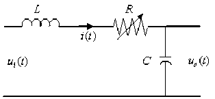
Fig 5.2 a nonlinear passive RLC network

So according to the output equation it is known that H 0 = { x ₂ } , by calculation, the smallest linear subspace H containing H ⁰ is

H = span { h , L f h } = span j x ₂, Cx_t

So the space dH has the constant dimension n= 2, which implies that parameter vector z = ( L , C , k ) can arbitrarily take values in parameter space, and the nonlinear system is observable, i.e., this system is structural observable.

Using Theorem 4.2 we also get the same result easily.

The output is y = x ₂ and the differential of output is

У = x 1 ]C . So the Jacobin matrix is as follows:

Г 0 1 ^ (y c 0 J

Obviously, the rank of this Jacobin matrix is 2, which is equal to the number of states, that is, this nonlinear system is structural observable.

Example 5.4 : We continue the example 5.3. In this case we add a separable sub-network on Fig. 5.2, which is shown by Fig. 5.3.

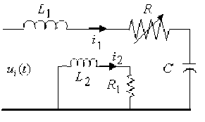
Fig 5.3 a separable nonlinear passive network

In the added separable sub-network L ₂ is a inductor and R ₁ is a constant resistance. So let the voltages across C and R ₁ be outputs denoted by u_{o 1} and u_{o 2} respectively. Then by KVL , we have:

L —+— l i d t + ki.² = u ¹d t C ^{J1        1}       '

< u01 = — [' dt o 1 CJ 1

L d - + R 1 i 2 = 0 j    d t

Let x 1 = i 1 ,x ₂ = u_o 1 , x ₂ = i ₂, u = u_t , y 1 = u 1 ,y ₂ = u_{o 2} , then the state equation and output equation is as follows:

;& ! =     u ^- x 2 ^- kx^)

L xK = - x

C 1

R

<  =—L x3

L 2 3

• У 1 = x 2

• У 2 = R 1 x 3

According to Theorem 4.2, we need to calculate the Jacobin matrix, which is of the following form:

r 0	1	0 )
0	0	R 1
1C	0	0.
0	0	- R 1 2 Il 2
- 2 kx1 /L 1 C	-1L 1 C	0
.     0	0	- R^l L 2 J

It is clearly the rank of this matrix is 3, and then the separable nonlinear passive network is structural observable; however, if we just chose the voltage across capacitor C as output, the separable nonlinear passive network is not structural observable. This is obviously because in the separable sub-network the state x ₃ is not observed by the voltage across capacitor C . Further more the whole separable nonlinear passive network is not structural controllable.

^ . CONCLUSIONS

In this presented paper structural observability of a class of nonlinear system is considered. Together with the conception of parameter space and indistinguishability of states the structural observability rank condition is defined and structural observability criterions of nonlinear system are obtained. No mater what methods used, i.e., differential geometry and algebraic method, the final work is to test the dimension of structural observability space. In fact the structural observability space is just the 1-form defined by space H in section Ш . If the parameters are indistinguishable, the solutions with the same time but different parameters are also indistinguishable. In section V it is known that these criterions can imply the well known rank condition for linear system, so these structural properties are more general and usful for nonlinear observability analysis.

A CKNOWLEDGMENT

The author wishes to thank professor Lu Kai-sheng. His some useful suggestion helps me improving this paper. His pioneering work in researching linear systems and electrical networks over F ( z ) makes me interested in structural properties research. The author also wishes to give his thanks to anonymous reviewers. This work was supported in part by National Nature Science Foundation of China under grant: No. 50177024.