Structural Identifiability of Nonlinear Dynamic Systems under Uncertainty

Published Online February 2020 in MECS

Definition 1. The system described by the equation (1) is called n -identified if the matrix A is possible to determine based on the measurement of the variable X .

Definition 2. The system described by the equation (1) call 1-identified if the matrix A possible to determine by of measurement y .

The n -identifiability condition consists in that the matrix [ X_o j AX₀ j A ² X ^ .. J A m -1 X J was nondegenerate.

1-identifiability conditions:

• 1.    The system (1) is n -identified.

• 2.    The pair ( A, C ) is observable.

• I.    Introduction. System Identifiability

The identification problem of dynamic systems despite the set of obtained results is one of relevant study directions. Fundamental results obtain on system parametrical identification. An approach to the identifiability estimation is base on R. Kallman ideas [1]. Further development of these ideas gives in [2, 3]. R. Li [2] gives the following identifiability definition.

Consider the system

X +1 = AX „ ,

Уп = ctX, where Xn e Rm is a state, A e Rmxm , yn e R is an exit, n = Jn = [0, N] is the discrete time.

Problem: determine by conditions under what the system is identified on the set

I _o = { У п , n = 0, N , N <» }            (2)

Following sufficient and necessary conditions are obtained in [2] when y_n e R m .

The identifiability case when the dynamic system order is less m consider in [2].

The considered result analysis shows that the identifiability estimation of the system (1) consists in the possibility of parameters identification. Designate by the parametric identifiability as IP identifiability (IPI). Many publications are devoted to the study IPI. The difference between these studies and the approach stated in [2] consists that identifiability results present in the form accepted in estimation problems of parameters. The concept of the structural identifiability introduced in [4].

Consider  two dynamic systems S ( U_x , Y_x , A ) ,

S^ ( Ui , Y , A ) with inputs U , U , outputs Y_x , У₂ and parameters A , A . Models    M_x ( U_x , Y , AL_X )     and

M ₂ ( U , Y , v A ₂) corresponds to this systems.

Definition 3 [4]. If the condition M_x (JA₁) - M ₂ (J A ₂) is satisfied at U_x = U₂ , Y = Y and ^A_x ^ J A₂ , then models are indistinguishable on observed inputs and outputs.

Definition 4 [4]. A parameter a_{x t} e A_x is called structurally globally identified if the condition

Ml ( A1 ) ~ M2 (A2 ) ^ a1,i = a2,i is satisfied almost for any A2 e ^p (except a zeromeasure subset of a parametrical space Qp).

Definition 5 [4]. A parameter a_{x t} e A_x is called structurally locally identified if such neighbourhood O^ ( A ) exists almost for any A e Q_p that

Ml ( A )“ M2 ( A2 )^ a1,i = a2,i follows from the condition A e O. (A).

The local identifiability is a necessary condition for the global identifiability. A parameter which is not structurally locally identified is called structurally locally not identified. Different approaches and methods apply for structural identifiability verification [5, 6].

In [7], a concept of local parametrical identifiability is introduced and given it’s the theoretical justification. Consider the system described by the vector differential equation

X = F(1 , X , P ), X ( 1 0 ) = X 0

where X_n e R m is a system state, P e R m is a parameter vector, F ( • ) is a nonlinear vector-function.

Definition 6. The system (3) is called locally identified in a point P e W if such г >  0 exist that couple { P , P } is distinguishable for any point P such that 0 <| P - P ol |< г .

Remark 1. System structure estimation methods not considered in most papers. Therefore, the structural identifiability concept does not reflect the essence of the considered problem. As this terminology applies in identifiability estimation problems, we will hold to this concept in this section. Further, we will introduce a concept which is directly related to the structural identifiability of nonlinear systems.

In [7], criteria of the linearized system (3) local identifiability estimation proposed. The case is considered when the matrix rank is equal m . The local identifiability estimation method based on the Lyapunov exponent analysis proposes for an inhomogeneous linear system. Parametrical identifiability criteria introduce in [8], and also given generalization and development of results obtained in [7]. Full identifiability conditions propose for a linear stationary system on discrete measurements of output and state variables in [9, 10].

The IPI-identifiability problem of nonlinear systems studies by many authors (see, e.g., [9-12]). In [10], the identifiability research base on the sensitivity system analysis on the output system. This approach efficiency illustrates in the example of the identifiability estimation of system parameter combination. This approach gives a new method the local identifiability problem solution. Local parametrical identifiability conditions obtain for different variants of the experimental data measurement in [9]. Conditions of joint observability and the identifiability obtain for the linear stationary system. The critical analysis of the approaches applied to the biological model identifiability estimation given in [11]. Models for the nonlinear system identifiability estimation based on the applying by the expansion into Taylor series, tables of identifiability (contains nonzero members of Jacobian coefficients row), the algebra of differentials. Paper [12] considered to the practical identifiability study. Practical identifiability estimation bases on the experimental information analysis and the differential algebra application. The basis of the practical identifiability is the leastsquares method and the model sensitivity analysis to the obtained parameter estimations. The proposed approaches apply to biology problems.

The identifiability of a static model considers in [13]. The model described by simultaneous equations system

BY +Г X n = U_n             (4)

where B e R^{m x m} is a nonsingular matrix, X_n e R k is an exogenous vector (external) variables, U_n e R^m is a vector of random external disturbances, Y e R^m is a vector of endogenous variables, Г e R^{m x k} .

The a priori information contained data about external and internal variables, properties U , restrictions on coefficients.

Consider the structure S = ( B , Г , M_n ) of the model (4) where M is a distribution U . Then Y at specified X have a distribution P^S .

Definition 7. If P S = P S , then frameworks S , S are observably equivalent.

Definition 8. A parameter Л is identified in the framework S if Л = Л is true for framework S = S .

So, the parameter Л identifies if Л = Л follows from equality P „ ^S = P S ( n = 1,2,..., N ).

Definition 9. The structure S is called identified if all its parameters identify.

Various cases of the a priori information accounting about S are considered in [13] and identifiability conditions obtained. They are restrictions on the rank of a matrix and depended on variables the system (4) which is normalized. The normalization is the solution of the equation (4) concerning Y .

Remark 2. Though the system (4) is static its studying is relevant for the identifiability problem. Here the concept structure is also used. Therefore, the existing interpretations and problem statements of the SI will be useful to compare.

So, the analysis of publications shows that the model identifiability is the estimation possibility of its parameters. The proposed methods base on the non-degeneracy estimation of an informational matrix. Similar results obtain in the parametrical estimation theory, and nondegeneracy condition (rank completeness) of the informational matrix is presented in easily checked the excitation constancy condition of the input and the output system. As a rule, the model structure specifies a priori, and the sense of the local structural identifiability is understandable not always. The structure concept widely applies in identifiability estimation problems. The nonlinear system identifiability also transformed into the parametrical identifiability problem on the base by the different methods linearization model application on parameters. These researches do not include the structural identifiability problem of nonlinear dynamic systems in the following sense: have the problem solution of the structure (a form, dependence) estimation a nonlinear system under uncertainty. The task not set was in this form.

Identifiability structural aspects of the nonlinear system consider in such statement in this paper. Identifiability structural is the complex problem, methods of structure formalization are not developed. The concept of the structural identifiability ( h -identifiability) introduce for nonlinear systems in [14]. The proposed approach directs to the structure estimation of the nonlinear dynamic system. It bases on the analysis of the framework described the state of the system nonlinear part. We are generalized results of paper [14]. The IPI-identifiability problem not considers. It’s the decision can obtain, having applied approaches described above.

The paper has the following structure. The problem statement is given in section III. The framework design method stated in section IV. The method describes the formation of a set for the construction S -framework. Framework class properties consider. Estimation need of the nonlinear system h -identifiability is substantiated in section V. System examples with hysteresis considered and the input parameters affect studies on properties of the nonlinear system. We show that the input has the constantly excited properties. But not every input that has excitation constancy property gives the solution of the structural identifiability problem. Bases of the nonlinear system h -identifiability (structural identifiability) describe in sections VI, VII. We introduce the concept of a system S-synchronization which the fulfillment allows solving the problem h -identifiability. The input which does not have property the S-synchronizability property gives to an "insignificant" S -framework. Structural identifiability estimation methods consider. We show that the h -identified framework S have a specified dimension. Numerical modeling results present in section VIII.

• II.    Related Work

Now, the structural identifiability problem of nonlinear systems reduced to the parametric identifiability problem [9-12]. Approach to the PI estimation has been proposed in [2, 3]. The development this approach considers in [310, 13]. This SI concept does not apply to the task set in the penultimate paragraph of section I. Non-traditional methods should apply to the SI problem solution of nonlinear systems. Such an approach based on the analysis of virtual frameworks proposes in [14]. The structural identifiability problem solution is given for the case when nonlinearity satisfies the sector condition [16]. We the identifiability concept and the condition of full structural identifiability ( h -identifiability) are generalized. The condition h -identifiability is satisfied if the system is S-synchronized.

• III.    Problem Statement

Consider dynamic system

X = AX +Bϕϕ(y)+Buu, y=CTX, where u∈ R, y∈ R are the input and the output, A∈ Rq×q; B∈ Rq , B∈ Rq C∈ Rq are matrices of corresponding dimensions; ϕ(y) is a scalar nonlinear function. A is the Hurwitz matrix.

Various assumptions made concerning the structure χ = ϕ ( y ). They determined by the a priori information level. Methods based on linearization procedures [15] can apply under the a priori information. The assumption concerning the function χ specifies in the absolute stability theory in the form

χ ∈ F ϕ = { ϕ ( ξ ) ξ ≥ ξ ², ξ ≠ 0, ϕ (0) = 0 }       (6)

where ξ ∈ R is the input of a nonlinear element.

ξ is the linear combination of vector elements X . The sector condition [16] is generalization (6)

χ ∈ F _ϕ = { γ ₁ ξ ² ≤ ϕ ( ξ ) ξ ≤ γ ₂ ξ ², ξ ≠ 0, ϕ (0) = 0, γ ₁ ≥ 0, γ ₂ < ∞ } .

Often the system (5) nonlinear part is described by static (algebraic) equations. Therefore, further, we consider a case when ϕ ( y ) describe by the algebraic equation. We believe that the function ϕ ( y ) is smooth.

Let the informational set be known for the system (5)

I o = { u ( t ), У ( t ), t ^G J = [ t 0 , t k ] }             (8)

Problem: estimate the structural identifiability of the system (5) nonlinear part by the analysis and processing I o

Identification parametrical methods application under uncertainty does not allow obtaining the SI problem solution. Therefore, we apply to the estimation of structural identification the approach proposed in [14]. The approach based on the design of the framework S reflecting properties of the nonlinear part (5). This analysis associated with the system structural identifiability problem solution. We use the term h -identifiability (HI) to distinguish the proposed approach from IPI-identifiability. Describe the design method of S -framework.

• IV.    Design Method S -framework

Design S -framework demands the preliminary formation of the set which contained the information on the function ^ ( y ). Describe to the obtaining Тд, method¹.

• A.    Set for Formation S -framework

Apply the differentiation operation to y ( t ) and designate the obtained variable as x . The consideration x expands of the system informational set: I_{e nZ}= { I_o, x } .

Remark 3. If variables u , y measure with an error, then apply to variables the filtering procedure.

Allocate a subset I gc I^ corresponding to the system (5) particular solution (steady state). The set does not contain data I on the transition process in the system. Apply the mathematical model

% ( t ) = H [ 1 u ( t ) y ( t )f               (9)

for the selection of the linear component in x . The variable x, define on an interval J = J \ J,, . H g R ³ is the

• 1                                                g             tr

model parameter vector.

Determine by the vector H as the task solution min Q (e )|    ^ H

H ^ ' | e=x| — X1        opt where Q(e) = 0.5e2.

Find by the prediction for x having applied by the model (9) and obtain the error e(t) = x’ (t) - x (t)■ e(t) depends on the nonlinearity ^(y) of the system (5). So, the set

1 n,g ={ У(t), e(t) t G Jg } obtains. Next, we apply the designation y(t) believing that.

Remark 4. The structure model (9) choice is the system (5) structural identification stage. Modeling results show that the model (9) is applicable in identification system objects with static nonlinearities. The structure model (9) choice for the system with complex nonlinearity presented in [14].

• B.    Frameworks S

Application of the phase portrait S described by function Г : { y } ^ { y '} not always the conclusion allows making about system nonlinear properties under uncertainty. Therefore, use the set I and go in the space Pye = ( У , e ) which we will call structural.

Consider the function Г : { y } ^ { e } which describes the change framework S on the plane ( y , e ) . I contains information on cp(y ) , therefore, S describe the nonlinear function change in a generalized form. The system (5) input has to satisfy certain conditions for the representation obtaining of ^ ( y ). It is the excitation constancy property. Such input gives to the closed framework S_ey .

• V.    About Need h -identifiability Estimation for Nonlinear System

• 2.2   if ( y - d >  2.2 ) &  ( y '> 0 ) ,

The review on the SI shows that the IP-identifiability problem is the main in SI. That the urgency of h -identifiability problem understands consider arising tasks on the example of the second order system (5) with parameters:

01       0

A = _₃  _₄ , B_u = B , = j , У (0) = 3, У ' (0) = 2

y - d if ( y - d <  2.2 ) &  ( y '> 0 ) ,

. 1.5 if ( y <  1.5 ) &  ( y '< 0 ) ,

y

a) frameworks

b) nonlinearity

Fig.2. Structure estimation results for u   ( t ).

2,2

2,0

Ф б, - 4⁽ У )

1,8

1,6

1,0   1,5   2,0   2,5   3,0   3,5   4,0

1,4

y

b) nonlinearity

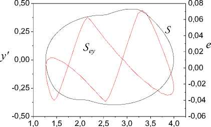
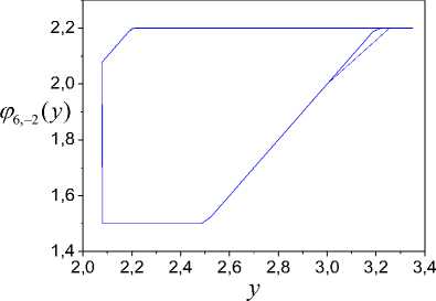
Fig.1. Structure estimation results for u ( t ).

Results presented below base on the application of the approach from section IV. These results show the input u ( t ) influence on the system (5) nonlinear properties. System properties estimate by the framework S analysis and the recovered function ф ( y ) corresponding to the input u ( t ) present.

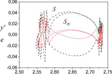
Fig. 1 represents the phase portrait S and the framework S for u₆ ^( t ) = 6 - 4sin ( 0.1 n t ) , and also the function ф ( y ) recovered from data { y ( t ), y ' ( t ) } . We consider the case of the established motion. Fig. 1 shows that u ₆ ^( t ) give to reference function ф ( y ) . The framework S is almost symmetric and has features which are in the framework S also.

2,0  2,2  2,4  2,6  2,8  3,0  3,2  3,4

y

a) frameworks

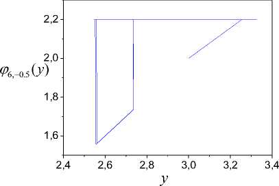
The further decrease of the sinusoid amplitude gives to the loss of the framework S symmetry feature. The restoration impossibility of the form function ф(y) is the result of such input property. Such function ф(y) resented in Fig. 2 when u6 2(t) = 6-2sin(0.1nt). We see that the sinusoid amplitude decrease gives to framework definition range compression and the framework left part to have more modification. Such input gives function ф6 2 (y) saturation area reduction. This area is not recoverable by the identification method application. Cardinal changes ф(y) gives u6 05 (t) = 6 - 0.5sin (0.1nt)

Corresponding results are shown in Fig. 3.

The modeling result analysis shows that input u ( t ) parameters are at which the structural identifiability (structural identification) of the nonlinear system is possible. These results present for the system with ® = 0.1 n in Fig. 4 where following designations use: D , D are diameters of the variation domain y , e ; a is the sine amplitude.

y

a) frameworks

b) nonlinearity

Fig.3. Structure estimation results for u ( t ).

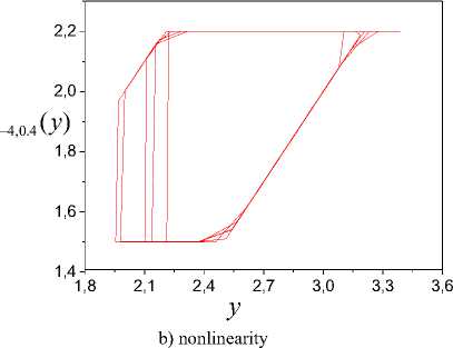
Fig.5. Structure estimation results for u ( t ).

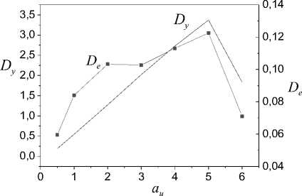
Fig.4. Input amplitude effect on the system (5) identifiability

Fig. 4 shows that the input ( a_u = 5 )exist which the SI problem solves. The system (5) (see Fig. 1) is identifiable with the input having the amplitude a_u = 4 .

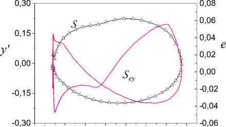
We considered the input amplitude effect on system features. Similar to the effect gives to the frequency influence (Fig. 5).

Remark 5. Modeling results show (Fig. 5) that ensuring the excitation constancy (EC) condition for u ( t ) can complicate the system h -identifiability estimation. Presented results show that requirements of the EC for the input have the essential distinction in structural and parametrical identification problems. It should be taking into consideration when the problem of active identification solved.

2,25

1,50

0,75

y'

0,00

-0,75

-1,50 1,8

S’ ey

S

2,1

2,4

2,7

3,0

3,3

y

a) frameworks

0,150

0,075

0,000 e

-0,075

-0,150

3,6

Modeling results allow giving to h -identifiability problem statement as the following task solution: find such an input u(t) for the system (5) which gives the definition range maximum for the output y(t).

• VI.    h -identifiability

Results obtained in section V show that methods applied to the IP-identifiability estimation do not work in the case the h -identifiability. Further, we state to the approach to HI estimation².

First, consider properties of the set I allowing the problem h -identifiability to solve. The analysis I gives properties of the informational set I determining a capability the consideration problem solved.

Let following conditions be satisfied.

• B1.    The set I gives the parametrical identification problem solution for the model (5). It means that the input u ( t ) is excitation constancy.

• B2.    The input u ( t ) given the informative framework S^ (^ g). It means that the analysis S^ gives the estimates task solution of system (5) nonlinear properties.

Definition 10. The input u ( t ) we call representative if it satisfies conditions B1, B2.

Let the framework S close, and its area is not zero.

Designate a height S^ as h ( S^ ) where the height is the distance between two points on opposite sides of the framework S .

Statement 1 . Let 1) linear part of the system (5) is stable and the nonlinearity ф(-) satisfies the condition (7); 2) the input u ( t ) is limited piecewise continuous and CE; 3) such 5 _S >  0 exists that h ( S^ ) >  ^ . Then the framework

S identifiable on the set I .

Definition 11. Framework S having specified properties is h - identifiable.

Let the framework S be h - identifiable.

Concept h -identifiability features.

• 1.    h -identifiability is a concept not parametric, and the structural identification.

• 2.    The demand of the parametric identifiability is the h -identifiability basis.

• 3.    h -identifiability makes more rigid demands to the system input.

Feature 3 means that "the bad" input can satisfy the excitation constancy condition. Input can give so-called an "insignificant" S -structure ( NS -framework). But the NS -structure can be h -identified. The identification of the system which has the property of insignificance can give to the nonlinearity which atypically for the examined system under uncertainty.

Consider the existence conditions of the NS -structures. Consider a class of nonlinear functions to which the homotopy operation is applicable. The homotopy [17] is the operation of obtaining one part of a geometrical figure from another part by it’s the rotation and the extension about a specific point on the plane ( y , e ).

Consider the framework S . Let S„, = Fl и FГ , ey               ey      Sey       Sey where Fl,Fr are left and right fragments S . Determine for Fl,Fr secants Sey    Sey

V s = ay , V s = a r y           ⁽¹⁰⁾

where a^l , a^r are numbers computed using the leastsquares method (LSM).

Theorem 1 [14]. Let i) the framework S is h -identified; ii) the framework S„, has the form S„, = Fl и Fr , ey                                   ey        Sey        Sey where Fl, Fr are left and right fragments S ; iii) secants for Fl,Fr having the form (9). Then S is NS -Sey    Sey                                                        ey            ey structure, if

II A -I a^r || >  5 h                  (11)

where di , >  0 is some specified number.

Remark 6. The theorem 1 proves used the homotopy of sets [17]. Estimate the proximity of sets Fl,Fr in this Sey    Sey case.

Remark 7. NS -structures are characteristic for systems with multiple-valued nonlinearities. They are the result of the inadequate application of input actions.

Consider the framework S . Introduce designations:

D_y = dom ( 5^ ) is the definition range S_ey ,

D y = D y ( D y ) = max У ( ¹ ) - min У ( ¹ )

is the diameter D . Let u ( t ) e U, where U is the permissible input set for the system (5).

Definition 12. If the framework S has the maximum diameter D_y on the set { y ( t ), t e J } , then the system (5) have S- synchronizing input u ( t ) e U .

We understand the synchronization u (t) e U as the choice of such input uh (t) e U which allows reflecting all features Sey characteristic for ^(y). It is true if u(t) ensures max D . Here the uh (t) e U and input property uh      y                        h choice is directed to the possibility of obtaining the framework S^ * NS. The proposed concept of the synchronization by differs from oscillation theory terminology. As the choice uh (t) e U can interpret as the synchronization between model and system structures, then dh = max D ensures the system h -identifiability.

, y         _{u h}        y

Let the input u ( t ) synchronize the set D . We will write u_h ( t ) e S if u ( t ) is S-synchronizing. Notice that the finite set { u_h ( t ) } e S exists for the system (5). The optimum choice u ( t ) depends from d . Ensuring this condition is a prerequisite of the system (5) structural identifiability.

Definition 13. If S is h -identifiable and the condition ||ar | - | a^r ||< 5_h is satisfied, then the framework S^ (the system (5)) is structurally identifiable or h -identifiable.

Definition 13 shows if the system (5) is h - identifiable, then has the area D of the framework S the maximum diameter. Let the framework S contain m features. We understand function ф (y ) features as the continuity loss on some interval, and function inflection points or a function extremum. These features are signs of the examined function nonlinearity.

Definition 14. If the framework S is h -identifiable, ey        °h then the model (9) is SM -identifying.

Theorem 2 [14]. Let 1) the input u(t) is constantly excited and ensures the system (5) S-synchronization; 2) the system (5) phase portrait S has m features; 3) the S -framework is h -identifiable and has fragments corresponding to phase portrait S features. Then the model (9) is SM -identifying.

The theorem 2 shows if the model (9) is not SM -identifying, then the model (9) structure or an informational set have to be changed.

Consider the framework S . Designate the framework S center on the set J = { y ( t ) } as e_s , and the area D centre as с .

D _y

Theorem 3. Let on the set U of the system (5) (i) such e >  0 exists that | e ₅ - e_D |< e ; (ii) the condition ||al | -| a^r ||< O satisfied. Then the system (5) is h_5h -identifiable and the input u_h ( t ) e S .

Proof of Theorem 3. Consider the input u_h ( t ) e U . As the condition | a ' - a^r | <  O is satisfied, the framework S is symmetric concerning the point с on the plane ( y , e ) . Therefore, fragment F^l_s , F_s r definition range diameters coincide within some size e >  0 on the set { У ⁽ t ) } , i.e.

I ^D< ( D . ) " D .- ( ® J|< ^e -

where D l , D r are ranges of definition F^l , F^r . F _S      F _S                                         S ey    S ey

The framework S centre is e_n = 0.51 D + D , I. As ey                  ^D y              F _S^l       F _S ^r

D , + D , = D such e >  0 exists that e„ - e_n <  e . Ful-

FSlFSry                                       S     Dy fillment of conditions (i), (ii) guarantees u(t) = uh (t) and dh = max D . Therefore, the framework S at uh (t)

,y       uh      y                                                       y will contain all features characteristic of the function ^(y). It follows that uh (t) e S, and the system (5) is h^ -identified.

Some subset {uh , (t)} c U6 c U ( i > 1 ) which elements have the S-synchronizability property can exist. The framework S^; (uh t) with the diameter D s of definition range D corresponds to every u(t) . As uh; (t) e S the diameter D , property. Let the framework S diameter d .

h ,z has the d -optimality of the system (5) has the

Definition 15. The framework property on the set U , if |d h ,z - D y ,J < e V i = 1,#U h .

S ey , i has d_h , _z -optimality it is such e >  0 that

Definition 16. Let the input subset { u_{h z}( t ) } = U₆ c U ( i >  1) exist which elements u_h; ( t ) e S , and frameworks Sey i ( Uh i ) corresponding to them have property d_{h z} -optimality. Then frameworks S^; ( u_{h t} ) indistinguishable on sets { ^u _h , i ⁽ t ) } , J y ( u ( t ) = u h,i (t ) ) = { y_h ,i (t ) } .

From definitions 15, 16 we obtain if the set U exists then the h -identifiability estimation can determine on any input u ( t ) c U₆.

Remark 8. Here, the cases of symmetric nonlinearities consider. Therefore, remarks made above about the NS -framework existence remain are fair. If a nonlinear function does not have the symmetry property, then the research of this problem to be continued needs. Explain it with nonlinearity features. The accounting of these features is possible only under a priori information on the system or the further analysis of the framework S .

Go to h -identifiability estimation methods of the system (5) now.

• VII.    Approach to h -identifiability Estimation

O h

Consider the definition problem of an integral indicator for the evaluation of h -identifiability. The problem base on the analysis of framework S properties.

In the nonlinear dynamics and the fractal theory, approaches based on the principle of the covering [18] apply for the dimension estimation of a framework. Different types of the dimension propose. Topological dimension is one of the primary indicators. The dimension estimates the framework geometry and is always indicates its internal features. Attractors and fractals often are heterogeneous. The heterogeneity characterized an irregularity of point distribution on the framework. Heterogeneity estimations of frameworks obtain by parameters reflecting of system properties. The heterogeneity reflects discrepancy between probabilities of the fractal filling with the specified bodies and geometrical sizes of the respective areas. Such heterogeneous fractal objects called multifractals [18]. S -framework of the dynamic system with many-valued nonlinearity is an example the heterogeneous pattern. Section V contains examples of such frameworks.

Various indicators of the covering (correlation dimension, informational dimension, etc.) are approximate and labour-consuming [18]. They assess of framework fragment geometrical distinction not always. Therefore, we introduce the integral indicator of the framework which is the distribution function of the variable e on the set { y ( t ) } [14]. Such an approach eliminates various a priori assumptions concerning the framework covering. State to the proposed approach.

Let the framework S  obtained for the system (5).

Perform the fragmentation S^, = Fl u FГ  where Fl , ey       Sey        Sey                   Sey

F ^r are left and right parts of the framework S . Fragments F^l , F^r described by functions e^l ( y ), e^r ( y ) where { e } c { e }, { e r } c { e }.

Construct frequency distribution functions (histograms) H^l , H^r for F^l , F^r . Obtained cumulative frequency functions IH^l , IH^r on the basis H^l , H^r . Let

I_% = { i A e , i = 1, k } is the definition range of functions.

Present the value range of functions Hl,Hr in the form of vectors

L (IHl) = [ IHl, IH.,..., IH| ] T r ( ih r)=[ih; , IH2;,.., H ] T

Here, k is the number of pockets set on I^ , A e is the pocket size on e .

Apply the model linearity form. You can supplement results obtained by statement 2 with the histogram analysis for the framework S . Obtain Hl,Hr and IHl,IH r functions and analyze their correlations considering features S . Some approaches propose in [14].

• VIII.    Examples

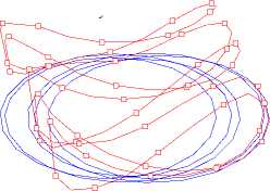
Consider the system from section V with the input u.(t ) = 6 - 4sin ( 0.5 n t ) + 0.4sin ( 0.1 n t ) . Frameworks S , S shows in Fig. 5 for system steady state. We see that conditions of theorem 3 are not satisfied. The sector which the function f_e = e ( y ) has to belong does not exist for S . Therefore, the system is not S-synchronized and S^ = NS . So, the system is not h - identifiable.

Let u(t ) = 6 - 2sin ( 0.1 n t ) . The system has frameworks showed in Fig. 2. Construct segments F^l , F^r for the framework S . It can be made by Fig. 2. Secants for F^l , F^r have the form S ey      S ey

Y _s = - 0.0359 y + 0.0792 , / r = 0.0211 y - 0.0649. (14)

R = a_HL ( IH^l )                (13)

and determine the parameter a having applied the leastsquares method.

The model is adequate if the parameter a_H g O (1) where O (1) is the neighbourhood 1. If the condition a_H g O (1) is fair, then the system (5) is h₅ -identifiable and S^ ^ NS_e . Otherwise, the framework S^ is insignificant.

So, the following statement is fair.

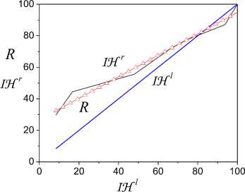
Fig.6. Estimation h -identifiability of system on basis fragment cumulative distribution function.

Statement 2. Let for the system (5): 1) the framework S^ = F u F_s r is defined on the set { y ( t ) } where

Fl,Fr is framework S ; 2) frequency Hl,Hr and Sey    Sey                                  ey cumulative IH l,IH r distribution functions are known for Fl, Fr. Then the system (5) is h -identified if aH g O (1) .

Definition 17. If the system (5) is h -identifiable, then the framework S_ have the dimension DH. = a_H .

ey              hH

Definition 17 shows if u(t ) g S, then dimension for the structurally identified system is approximate to 1. Such value DH shows that the framework S does not have complex areas and fragments F^l , F^r are structurally identical or homothetic. If DH_h £ O (1), then it is a sign NS -framework or a system with more complicated non-

Application of the theorem 1 shown that S^ = NS^ , i.e. system is not h -identifiable. This conclusion confirmed with diameters D _T = 0.478 , D _r = 0.792 . h -

FSl , FSr identifiability estimation results of the system shown in Fig. 6. They base on the application of statement 2. The model (13) has the form

J R = 26 + 0.656 L ( IH¹ ) .            (15)

The determination coefficient of the model (15) is equal to 97% that confirms the model adequacy. The framework S dimension is 0.65. Analysis results show that the system (5) is structurally non-identifiable on input u (t ) = u ₆,-4 ( t ).

Consider the system from section V with u (t) = u6 _д( t) = 6 - 4sin (0.1nt).

Corresponding frameworks showed in Fig.1. We see the framework S have some asymmetry that explains with characteristics of the nonlinear function (Fig. 1b).

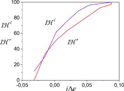
Fig.7. Functions IH ^l , IH ^r .

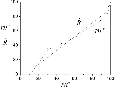
Fig.8. Estimation h -identifiability of system on basis fragment cumulative frequency function with u ( t ).

Following parameters of the secants (10) obtained for fragments F l , F^r r  : a¹ =- 0.025 , a r =- 0.027 . Let

S ey     S ey

^ = 0.003 . The condition (11) not be satisfied and 5 ^ NSe. To confirm this inference, determine by func tions IH l, IH r. They showed in Fig. 7, and results S -framework dimension estimation presented in Fig. 8.

The model (13) has the form

R = - 5.845 + 0.96 L ( IH¹ )

and the coefficient of determination is 96%.

Conditions of statement 2 satisfied and the system is h -identifiable. Framework S dimension DH is 0.96. ° h                                               ey                           h

Diameters of framework fragment are equal D^ = 1.16,

D , = 1.43. The diameter S is equal 2.59. This value

F r                                          ey coincides with D , + D , . If to choose e = 0.4, then the FSl       FSr                           F           , condition (12) will be satisfied. The distinction between fragment Fl,Fr definition ranges depends on properties Sey    Sey

S . The condition 2) theorem 3 satisfies with e = 0 . Therefore, the system is the SI or h -identifiable with u 6, - 4 ( t ), and u 6, - 4 ( t ) e S .

Generalizing above stated, obtain the following procedure of structural identifiability applying. Apply proposed methods at the initial stage of the model structure choice. Obtained results answer to the question: whether the system model has the nonlinear structure. The successful solution of this task depends on the properties of the input. If the input has the property of constant excitation, then apply procedures to design frameworks S , S . Perform the analysis on the estimation h -identifiability of the system and make the decide on the application of the nonlinear dynamic model. Further, apply parametrical identification methods and obtain model.

Proposed methods and algorithms applied to the structural identification (structural identifiability) of the system with RC-OTA oscillator. Verification of obtained results confirmed the structural identifiability of the considered system based on the structurally-frequency method application.

• IX.    Conclusion

The works analysis shown that the structural identifiability of nonlinear systems estimation based on parameters estimation. This approach does not allow solving the identifiability problems of nonlinear systems. In particular, it does not allow to obtain the solution of the nonlinear system structural identification problem under uncertainty. The approach proposed in this work is the basis for the solution of the structural identifiability problem. We have shown that the input has to satisfy the excitation constancy condition. This condition differs from requirements to input in adaptive systems. The system S-synchronizability concept is introduced. The solution of the structural identifiability problem base on frameworks analysis. Therefore, the ensuring of S-synchronization give to the maximum value of the framework definition range and the problem SI solving. Non-synchronized input gives to an insignificant framework which does not allow solving the structural identification problem. Therefore, the system is not structurally identifiable. We obtained conditions under which it is possible to estimate the system structural identifiability. The structural identifiability estimation method is proposed. We have shown We have shown that the subset of inputs which have the S-synchronization property exists, but frameworks are indiscernible on this subset.