Structural-parametrical design method of adaptive observers for nonlinear systems

Design of adaptive observers is one of the rapidly developing areas of control theory. The basis of theory AO for the linear class of dynamic systems has been obtained an end of past century [1-5]. The first direction [1-5] is based on reduction of the system to a special identification representation with use of auxiliary variables in space "input-output" (non-canonical identification form). Results obtained in [1-5] are the basis for the development and generalization on the theory to new system classes. Studies in this area continue. In particular, design methods of AO are generalized on time-varying system class. Many works give to generalization of obtained results on nonlinear systems. First results on design of AO for nonlinear systems were obtained in [6]. The observer canonical form for nonlinear time-varying systems is proposed. The structure of the system nonlinear part is necessary known and depends on a set of unknown parameters. The adaptive observer application for the solu- tion of different tasks is shown. Further development of the canonical form on the nonlinear case is given in [7, 8]. Application results obtained in [7] are given in [9]. Three adaptive nonlinear output-feedback schemes are presented in [9]. The first scheme employs the tuning functions design. The other two employ a novel estimation-based design consisting of a strengthened controller-observer pair and observer-based and swapping-based identifiers. Nonlinearities are smooth and known. The method of Lyapunov functions is applied to design of adaptive algorithms. Indirect adaptive control [10] is used to regulating system design of saturation rate. The stability of the adaptive system is proved. The adaptive gradient algorithm is applied to the tuning of an unknown parameter vector. Application of the adaptive observer is given in [11] for the control a linear system with a nonlinear parameterization of the saturation.

The design method AO for a nonlinear system based on applications B -splines is proposed in [12]. It is supposed that the nonlinear part depends on unknown constant parameters. It is showed that the proposed approach allows reducing the number of auxiliary filters. Robust design AO under the influence of disturbances and modelling errors is considered in [13]. The variation domain for system parameters is known. The structure and parameters of the nonlinear part are also known. Nonlinearity linearization of the system is fulfilled and the projective algorithm is proposed for tuning of unknown parameters.

The second direction of AO design is based on the Kalman filter theory and Luyenberger structure. This direction is widely applied at design AO for nonlinear dynamic systems [14-17]. Paper [14] represents design method AO in the Luyenberger canonical form for fault estimate in nonlinear systems. The nonlinearity is known and satisfies the Lipschitz condition. The fault is described by an unknown nonlinear function which is approximated on the class of known functions. Application of the extended Kalman filter with adaptive gain was considered in [15-17]. The system nonlinear part is smooth and satisfies the Lipschitz condition. The nonlinearity structure is known. Convergence estimations of adaptive algorithms are obtained. Application of neural networks (NN) for the design of AO for the nonlinear object under restrictions is considered in [18]. NN realizes the linear approximation of the system nonlinear part.

Effect of uncertainty in measurements is researched. AO in the Kalman filter form is proposed in [20]. Adaptive algorithms for filter parameters tuning are obtained as the solution of linear matrix inequalities problem. The form of nonlinearities in the system is known and they satisfy the Lipschitz condition.

So, adaptive observers are widely applied to the solution of different problems. The nonlinearity in most cases is smooth and satisfies the Lipschitz condition. The nonlinearity structure is, as a rule, supposed known. If the nonlinearity form is unknown, then it is approximated on the specified class of functions. But the systems class is for which the a priori information is incomplete or is unknown. Application of approaches considered above demands fulfilment of labor-consuming studies. The design AO is associated with the structural identifiability (SI) of nonlinear systems. This problem was formulated in [21] and obtained the generalization in [22]. SI allows making decisions on a possibility of nonlinearity identification on the basis of the available information. Studies will show that requirements to parametrical and structural identification significantly differ. This problem was not studied. Identification approach is one of the main in these conditions. But successful application of the approach depends on structural identification results.

This paper contains the solution of specified problems. We propose the structural-parametrical method for design of the adaptive observer for nonlinear dynamic systems under uncertainty. AO has the canonical form proposed in [4, 6].

The paper has the following structure. In the section II we give to problem statement. Section III contains the structural approach statement to AO design. The main attention is give to system structural identifiability estimation on the basis of virtual framework analysis. The method and criteria for estimation of the structural identifiability are proposed. We consider the case of onevalued nonlinearities. The method for estimation of a class and parameters of the nonlinearity is proposed. It is based on the analysis of virtual frameworks S and sector sets [23]. Structural stage results are applied at the design of adaptive algorithms for AO (section IV). Information obtained at structural synthesis stage can be used in two cases. It defines the adaptive observer structure. The case 1 correspond the complete information about the nonlinearity. The Lyapunov functions method is applied to tuning algorithms synthesis of AO parameters. The case 2 correspond incomplete or approximate information about the nonlinearity. Uncertainty appearance in AO is the consequence of structural information incompleteness. The uncertainty estimation procedure based on the analysis of the current information is proposed. The stability observation system analysis is stated in the section V. Simulation results are presented in section VI. The conclusion contains inferences and discussion of the obtained results. The system adaptive observation stability proof is given in the appendix.

• II.    Problem Statement

Consider system

X = AX+A^^+Brr, y = CTX, where X e Rm is state vector; r g R is input; y g R is output; ф(y) g R is nonlinear function; A g Rmxm is Frobenius matrix

A =

"0 I I m -1 A 1

A g R^m is the vector of unknown parameters belonging to a limited area G_A ; A e R^m , A = [ О,...,О, а_ф ] , B_r g R^m , B_r = [ О,...,О, b_r ] T are unknown parameter vector; I_m_ j g R^{(m - 1) x ( m - 1)} is identity matrix; С g R^m , C = [ 1 О ... О ] T . A is Hurwitz matrix.

Assumption 1 . The input r ( t ) is constantly excited and limited.

Assumption 2. Function ф(y) is smooth, single-valued, and фе F = {К1^ ^ ф<-)- ^ K2^2, 5 * 0, .(2)

ф (О) = О, к ^ о, к < ^ }

The data set for the system (1) has the form

Io ={u(t),y(t) t g J = [tО,tk]} .

Apply to y , r , ф the auxiliary system

Px = Лр + Hv , v = y, r, ф,(4)

where Л g R ^{( m - 1) x ( m - 1)} is stable diagonal matrix; H g R m ^{- 1}, h = 1 ( i = 1, m - 1) . Pair ( Л , H ) is controllable.

Apply the mapping X = TX to the system (1) and obtain

X = AX + Афф + B r r , y = C T X ,

where T e R"^xm , A _ф = T"‘ A _p , B_r = T "1 B_r , A = T"‘ AT ,

A = A y

HT

„

Apply model for the identification system (5)

/V                     . /X           _      _ /X             /X                /X                 /V

X = AM (X - CC X) + AуУ + АфФ + Br (t) r, у = cx , where AM e Rmxm is the stable matrix of the form

A M =

- k

HT

Л

k >  0; A e R m , A ^ e R^m , B e R m are vectors of tuned parameters; X e R^m is state vector; у e R is model output.

Use the system (4) and transform equations (5) and (6) to the form y = AX + AX + BTPr,         (7)

У = - k ( у - у ) + A T P y + A , P , + B T P ,       (8)

where p = [ у ^р у ] ^T , p = X ^p ] ^T , p = [ r ^p r ] ^T .

Problem: for the system (7) satisfying to assumptions of A1 and A2 define by such laws of tuning A ( t ), A ( t )

and B(t) model (8) that lim|у(t)- у(t)| < Пу , пу > 0. t ^ro                        у

The design of AO is based on the implementation of two stages.

• 1.    Structural stage (SS).

• 2.    Parametrical stage.

SS gives to nonlinearity localization ср ( у ) . The result localization is the class F definition and structural parameter nonlinearity estimation. The parametrical stage based on SS gives to tuning algorithms for AO.

Next, we describe these stages.

• III.    Structural Stage

To basis of SS is structural identification (p ( у ) e F^ . We apply the approach and methods proposed in [21, 22]. The structural identification first step ensures the construction of framework S . It is based on obtaining of the set I _{N , g} .

• A.    Formation of Set I

The method for construction of set I is based on results of work [24]. Determine i -th by derivative y ( t ) and designate obtained variable as x . The account x expands the informational set I_o : I_e„_Z= { I_O, у } . Consider the data subset I _go I^ corresponding to the particular solution of the system (1) (steady state). We will form set I excepting a data I . I is information on transition process in the system. We have I = I_ent \ I_tr .

Apply the mathematical model xl (t) = DT [1 u(t) у(t)]T                 (9)

and obtain of a linear component x . The variable x is defined on the interval J_g = J \ J_tr . D e R ³ is the parameter vector the model (9).

Define by the vector D as arg min Q(e)  .z ^ Dnnt.

° D         e\x=-xl-Xz         oPt where Q(e) = 0.5e2.

Apply the model (9) V t e I . Find the forecast for variable x . and generate the error e ( t ) = .x¹ ( t ) - x ( t ). e ( t ) depends on the nonlinearity

( у ) in the system (1). We obtain set I^ _g = { у ( t ), e ( t ) t e J_g } which we use on the second step of SS. Apply the designation y ( t ), supposing that у (t ) ^e I n , g .

Remark 1. Structure choice of the model (9) is one of structural identification stages. Modelling results show that the model (9) is applicable in object identification systems with static nonlinearities.

Remark 2. The choice of variable x is defined by system properties.

The next step of the structural identification is based on framework analysis S and S reflecting a state of the system nonlinear part.

• B.    Construction of Framework S

Virtual frameworks (VF) S and S are proposed in [25] for the analysis and design of identification systems. Development and generalization of VF on static system class is given in [26]. We present the approach to design VF proposed in [22].

Let S is phase portrait of the system (1) described by function x = f (у) (у is first derivative у ). We analyze the system (1) in the space Pye = (у, e) . Call Pye the structural space. The framework S described by the function Г : {y} ^ {e} Vt e J is phase portrait of the system nonlinear part. S can be closed. It is characteristic property of a dynamic system. We will apply to decision-making also S -framework which is described by function ГЕк : {ks (t)}^{e(t)} , where ks (t) e R is the coefficient of structural properties [24, 25]

k ( t ) = e ( t ).

^s        y ( t )

The form and features of the framework S influence on identifiability nonlinear dynamic system. The analysis of features S led to the introduction of the concept structural identifiability. Therefore, consider properties of the set I on which the framework S is specified.

• C.    Structural Identifiability of System (1)

Consider properties of the set I ensuring the solution of the structural identification problem. First, the initial set I has to ensure the solution of the parametrical identification problem. It means that the input r ( t ) is to nondegenerate and constantly excited on the interval J . Secondly, the input ensures the design of the informative structure 3^ ( I_{w g}) (or 3^ ) guaranteeing to make decision on nonlinear properties of the system (1).

Call the input r(t) representative if the analysis S  al lows make the decision about properties of the system.

Let the framework S be closed. It to mean that area S is not zero. Designate height of the framework S as h ( 3^ ) . h ( 3^ ) is the distance between two points of opposite sides of the framework S .

Statement 1 [24] . Let: 1) the linear part of the system (1) is stable, and nonlinearity ^ ( - ) satisfies the condition (2); 2) the input r ( t ) is limited piecewise continuous and constantly excited; 3) such 5_S >  0 exists that h ( 3^ ) > 5_S . Then the framework 3^ is identified ( h -identified) on the set I .

We suppose what S have the specified property. Features of h -identifiability [22].

• 1.    h -identifiability is a concept not of parametrical, and structural identification.

• 2.    Parametrical identifiability requirement is basis h -identifiability.

• 3.    h -identifiability imposes more stringent requirements to the system input.

Feature 3 means that the "bad" input can satisfy excitation constancy condition. But such input can give to so- called "insignificant" S -framework ( NS -framework) [22]. NS -framework can be h -identified. The insignificance property under uncertainty gives to the identification of nonlinearity, atypical for the system.

Remark 3. Next, we will show that the "good" input can generate the S -framework which does not give to reliable structural parameters of nonlinearity. It means that the input has to give to the framework S with certain properties.

NS -framework . Consider a class of nonlinear functions to which homothety operation [27] is applicable.

Let 3_ = F u Frr , where Fl , Frr  are left and right ey       Sey       Sey                    Sey    Sey fragments S . Determine for Fl,Fr secants ey                                 Sey    Sey

Y s = a‘У , y S = a^ry ,              (10)

where a^l , a^r are numbers calculated by means of the least-squares method (LSM).

Theorem 1 [21]. Let: i) the framework S   is h - identified; ii) the framework S has the form 3„,, = Fil u F„r , where Fl , FГ are left and right frag-ey       Sey        Sey                    Sey    Sey ments; iii) secants for Fl,Fr have the form (10). Then Sey is NSey -framework if

| al - ar| > 5h, where ^ > 0 is some number.

Remark 4. NS -frameworks are characteristic for systems with many-valued nonlinearities. They are inadequate application result of input actions.

Definition 1. If the framework S is h -identified and the condition | a^r - a^r | <  ^ is satisfied, that 3^ is structurally identified or h -identified.

Let the framework S have m features. We understand features of a function f as the loss of the continuity on the interval I ^j flex points occurrence or extreme. These features are a sign the function nonlinearity.

Apply the model (9) and construct the framework S in the space P .

Definition 2. The model (9) is SM -identifying if the framework S is h -identified.

Theorem 2 [22]. Let: (i) the input r(t) is constantly excited and ensures the h -identifiability of the system (1); (ii) the phase portrait S of the system (1) contains m features; (iii) S -framework is h -identified and contains the fragments corresponding to features phase portraits S . Then the model (9) is SM -identifying.

The theorem 2 shows if the model (9) is not SM -identifying, then it is necessary to change the structure of the model (9) or informational set for its design.

Another approach is proposed in [22] to estimation h -identifiability of the system (1) It gives to solve the following problem:

choose on the processing basis of set I the integral indicator allowing make the decision about insignificance S -framework.

Apply this approach to decision-making on the nonlinearity class.

Consider system (1), and obtain the framework S . Fulfil the fragmentation S . Fragmentation conditions depend on the form S . Consider the simplest case when the framework has the form:  S^, = Fl u Fr  where ey       Sey       Sey

Fl,Fr is left and right parts the framework S . Func-Sey    Sey                                                                            ey tions el(y),er(y) describe fragments Fl,Fr where {el }c {e}, {er }c {e} . Construct frequency distribution functions (histograms) Hl,Hr for Fl,Fr. Obtain cumulative frequency functions IH l,IH r on basis Hl,Hr.

Let I_% = { i A e , i = 1, p } is definition range of functions H^l , H^r . Describe value range of functions IH ^l , IH ^r by vectors

L (IHl) = [ IH, IH2,..., IHp ] T,r ( ih r) = [ ihr, ih[,..., ihr ] T.

where p is the quantity of pockets set on I^ , A e is pocket size.

Apply the model to the distribution description of the right fragment S

RR = a_HL ( IH l ) ,

and determine by parameter a , applied LSM. R ^ˆ is model output. The model is adequate if the parameter a_H g O (1) where O (1) is neighbourhood 1. If the condition a_H g O (1) is true, then the system (3) is h₅ -identified and S_ey ^ NS. . Otherwise the framework S_ey is insignificant.

Statement 2 [22]. Let for system (1): 1) the framework

S^ is obtained; 2) S^ has the form 5^, = Fl u Fr , ey                                   ey                                ey       Sey       Sey where Fl, Fr are fragments of framework S  deter- mined on the set {y(t)} ; 3) frequency distribution functions Hl,Hr and cumulative frequency functions IH l,IH r are obtained for Fl,Fr; 4) the dependence between R (IHr) and L (IHl) has the form (11). Then the system (1) is h^ -identified if aH g O(1) .

Introduce D -dimension of the system (1) by analogy with fractals [22].

Definition 3. The system (1) have dimension D_h = a_H if it is h -identified.

⁵ h

Definition 3 will show that dimension is close to 1 for the structurally identified system.

Estimate the nonlinearity class of the system (1) on the basis of the analysis S .

• D.    Estimation Nonlinearity Class

Consider classes of one-valued F and multiplevalued F nonlinearities. These classes contain set of nonlinear functions. We will apply the approach to identification of the nonlinearity class [15, 16] based on the analysis of sector sets.

Fulfil fragmentation of the framework S , using a subset I c ^ _g . I^ reflects change of the function X = ; (y ) in P_ye . The obtaining algorithm I^ is described in [22]. We will consider case of single-valued nonlinearities.

Consider the fragment FR^ c S_ey defined on I i for 3 i >  1 , I,_p c I^ . Construct for FR¹_ф the sector set [15]. Apply the least-squares method and determine for FR ⁱ the secant

Y = Y ( y^(t ) ) = a_ty⁽t ) + b_t .            (12)

Determine by mean value y for y ( t ) on I¹ c I . Let y is the centre FR ф on I i c I . Draw the perpendicular from the point y to intersection with Y on the plane ( y , e ) . Set constant c_t >  0 and construct straight line in the point a = ( y , e ( y ) )

Y , - = a , - y ^{( t} ) + b i , ^Y i , + = ^a i, + y^(t ) ⁺ b i ,

where az;+(_} = a ± c..

^Let Sec a i ( ^FR ^ , ) = ( Y , - , Y , + ) is the sector set for FR and

Sec ( FR ; ) = Sec a , I ( TR ^ ) и Sec a , _r ( FR ; ) , where Sec _a , l ( fr ; ) , Sec _a , r ( fr ; ) are subsets Sec ( fR^ ^ )

located at the left and to the right of the point a .

Construct secants

К I = a i , 1У (t ) + b i, I , Y i, r = a i , гУ (t ) + b i , r        (13)

for each of the parts FR ⁱ of the fragment FR ⁱ belonging Sec _a , i ( FR , ) and Sec _a , _r ( fr , ) . Apply the modification of the statement from [15].

Let such ^ >  0 exist that

I a i, 1 — ^a i |< ^ , l a i , r — a |< S '             ⁽¹⁴⁾

Theorem 3 [28] . Let: (i) frameworks FR ⁱ are described by functions X ey , 1 ( r ) ^: { y } ,11 ( r ) ^ { e } , , 1 ( r ^{(ii) secants (12)} are obtained for X ,/(r) in the space P = ( y , e ) ; (iii) the fragment FR i have the secant (13) where { y}.   с I_p,

{ e }_/Z(r) с I i_p . Then the function ф (y ) e T_ov if it is satisfied (14), otherwise ф(y ) e T_mv .

The theorem 3 shows if conditions (14) are satisfied, then Holder-Lipchitz condition is fair for ф ( y ), and the homothety operation is applicable to sectors Sec « , 1 ( FR A ) , Sec „ , r ( FR A ) .

We suppose that the assumption 2 will satisfy. Therefore, ф (y ) e T .

• E.    Nonlinearity Structure Estimation

The structural identification problem of nonlinear systems under uncertainty is difficult. General approach is not developed for its decision. Each nonlinearities class has features. They influence by form system trajectories. Detection of these features under uncertainty gives to the analysis S^ or S_ek . As ф ( y ) e F_ov apply the algorithm AF and the theorem of 4 [22] to the estimation of structure and parameters of the nonlinearity.

So, the structural design stage of AO is finished. Go to the parametrical design stage of the adaptive observer.

• IV.    Parametrical Stage

This stage is based on localization results of the nonlinearity ф ( y ) obtained in section III. Consider two cases of information on ф ( y ) .

• Case 1.    We suppose that we have the complete information about the structure ф ( y ). Subtract (7) of (8) and obtain the equation for the error s = y - y

s = - k s + A A A ^ + A A A P , + NB^T r P r ,     (15)

^where A A y = Al y ^- A y , A A , = A ^- A , , ^A A = Ai r ^- A .

Apply Lyapunov function V (t ) = 0.5 s ² ( t ) . Determine V s

Vs = -ks2 + s(AATPy + AAy + ABPP„) , and obtain parameter tuning algorithms of the model (8) from the condition V < 0

AAy = Ay =-rysPy,(16)

AA, = Al, =-r,sP,,(17)

AAr = Ar =-ГrsPr,(18)

where Г e R m ^{x m} , Г e R m ^{x m} , Г e R m ^{x m} are diagonal matrixes with positive diagonal elements.

Designate the obtained adaptive system (15) - (18) as AS A .

Proposed approach differs from the results obtained in [7-10] use of the structure , ( y ) which is determined at the structural identification stage under uncertainty. It allows to applying known adaptive algorithms.

• Case 2.    A posteriori information about , ( y ) has approximate character.

Assumption 3. The structure , ( y ) is specified as the set

, e T _ov = { W e R : , ( y ) = F^T ( y , W_X)W₂, W = [ w ^t , W^T ] ^T , W e W„ } ,

where W_n = { w e Rⁿ : W <  W <  W } is the area formed posteriori; W , W are vector borders for W . Some elements W , W can be unknown.

• (19)    shows that the function ф (y ) have at this stage has the form

, ( y ) = F T ( y , W 1 ) W 2 ,             (20)

where W e W_a с Rⁿ is the vector of parameters ф (y ) .

We suppose that W=W u W₂ . The set w с R n ( w e W ) contains elements which are not tuned. Elements W e W₂ с R n ² are estimated on the basis of parameter tuning AO. The vector F ( y , W ) e R^{n 2} is formed at the structural synthesis stage AO. Explain representation (20) as the proposed parametrical concept for ф ( y ).

Therefore, the main difference from the case 1 is need of the current estimations obtaining for the vector W and for the nonlinearity ф ( y ) . The equation (8) is not applicable and is required to its modification.

Present model for the estimation p(y) as p (y) = FT (y, WW         (21)

where W , e R n ² is the tuned parameter vector; W e R ” ¹ is the estimation vector for W which are adjusted on iterative constraint. Next, we propose the constraint algorithm for W ^ˆ .

Apple (20), (21) and modify the adaptive model (8). Obtain the current estimation for the vector P :

P p  A / ^. + He p ( y ),             (22)

and rewrite the model (8) as y = -k (y - y) + ATPy + АТЛ + BiTPr, where P = ^Ф Рф ]  . Transform this equation that to perform association with the equation (7). Obtain y=-k (y - y)+A}P>y+AP+Btp ± \P =

• - k ( y - y ) + A T P + A T P p + В T P r + № ,

where № = -v. ( P - P p ) = a ; \ P p .

We see that the equation (23) contains uncertainty №. Use the approach proposed in [29] to the estimation №. Apply numerical differentiation and obtain the estimation for y . Designate the obtained variable as y(t). Apply model to the estimation y yd = ATP + ВTP,(24)

and determined by the misalignment ст = yd- yd. Rewrite the equation (23) as y = - k (y - y) + ATPy + A> + 6А'. с,(25)

where с is the current estimation № . The equation for the error 8 write as

• 8 = - k8 + AAPPy +AA;Pp + ABTP + с.(26)

Design adaptive algorithms for parameter tuning of the model (25).

Algorithms for A ^ˆ , A ^ˆ have the form (16), (18). Apply the Lyapunov function V_£ and from the condition V_g<  0 obtain the algorithm for A ^ˆ

.              /X                              /X

^ A p = A , = -Г _ф 8Р_ф ,            (27)

where Г_ф e R m ^{x m} is the diagonal matrix with positive diagonal elements.

Consider the Lyapunov function V_a (t ) = 0.5 с ²( t ). As с = № and

APp = AAPp + HFT (y, W)AW2

that obtain the algorithm for tuning W ^ˆ from the condition V <  0

/X                   /X „~

W =-Г2с.4THF ,(29)

where A P^, = P₉ - P , A W, = W, - W ₂, Г₂ =Г T >  0 is the matrix ensuring convergence of the algorithm (29).

Designate the adaptive system (16), (18), (21) - (29) as AS p .

Iterative constraint algorithm for the vector W ^ˆ .

• 1.    i = 0.

• 2.    Let W_;J = W * , where W * e W_a.

• 3.    Perform parameter tuning of the system AS .

• 4.    Check the condition lim| y ( t ) - y ( t )| <  n . If it is t ^да                        ^y

• 5.    i = i + 1.

• 6.    Suppose W ,z= W -1+ ^ W , where 5 W_X chooses from the condition W,i e W_a .

• 7.    Go to step 3.

satisfied, then finish the algorithm work, otherwise go to the step 5.

The case 2 has a difference from the case 1 and [7-10]. We suppose that at the structural identification stage identify the form p ( y ). But obtained values of parameters p ( y ) can differ from original parameters. It demands model parameterization for p ( y ) and algorithms design for AO parameters tuning. Obtained estimations of AO parameters are the basis for tuning of the auxiliary vector P ^ˆ and compensation of the appearing uncertainty. The filter structure for P ^ˆ is formed a posteriori. This is the main difference of the proposed approach from [7-10].

• V. Stability Analysis

Consider the system AS . Show to system trajectory limitation. Let A K ( t ) == |^A A T (t ), A A T ( t ), A B _r ^T ( t ) ] ,

V (t ) = 0,5 A K^T (t ) F ^{- 1} A K ( t ),          (30)

V (t ) = V _e (t ) + V _K (t ),               (31)

where F ^A F +Г +Г_Г , + is the direct sum of matrixes.

Theorem 4. Let: 1) functions

V ( t ) = 0,5 s ²( t ), V_K ( t ) = 0,5 A K^T ( t ) F ^{- 1} A K ( t )

are positive definite and satisfies conditions inf V ₆ ( s ) — ^ , inf V_K ( A K ) — ^ ; 2) assumptions 1, | s —^                          ||a k| I—^

• 2 for the system (1) are satisfied. Then all trajectories of system AS are limited, lie in the area

• G , = { ( s , A K ) : V ( t ) <  V ( t о ) } ,

and the estimation is fair

t

J 2 kV _E (t) d T <  V ( t о ) - V ( t ).

t ₀

The proof of Theorem 1 is given in the appendix A.

Theorem 1 shows that all trajectories of the adaptive system AS are limited. Ensuring the asymptotic stability demands the imposing of additional conditions on the system. Consider these conditions.

Let P(t ) ^A [ P T ( t ) p^T ( t ) P T ( t ) ] T , l = 3m .

Definition 4. The vector P e R ^{3 m} is constantly excited with level a or has the property PE_a if

PEa : P(t)PT (t) > all is true for 3 a > 0 and Vt > t0 on some interval T > 0.

If the vector P ( t ) has property PE then we will write P(t ) e PE a .

The system (1) is stable, and the input r ( t ) is restricted. Therefore, property PE present for the matrix B P (t ) = P(t ) P^T ( t ) as

PE a,a : a l l <  B p ( t ) <  a l l V t >  1 0 ,       (32)

where a >  0 some number.

Let the estimation for V ( t ) is fair

0.5 pp (F)||AK(t)||2 < Vk(t) < 0.5 Д"1 (F)||AK(t)||2 (33) where Д (Г), Д (Г) are minimum and maximum eigen- values of the matrix Г .

Proof of the exponential stability is based on ensuring M ⁺ -property for functions V ( t ), V_K ( t ) [30].

Definition 5 . The non-positive quadratic form W ( Y , X ) has M ⁺ -property or W ( Y , X ) e M ⁺ , if it is representable as

W (Y, X) = -cv|Y| I2 + Cx||X| I2, for any Y e Rm, X e R” in the restricted area Qp, where cx > 0.

Lemma 1. V ( t ) have M ⁺ -property

• •          ae (f)

V < - kF + ^P *^v ’ V_K .             (34)

• ^{6       6}       k ^K

The proof of Lemma 1 is given in appendix B.

Lemma 2. V_K ( t ) have M ⁺ -property

V k <- 3 9ap i ( Г ) V _K + 8 9 V 6 .         (35)

The proof of Lemma 2 is given in appendix C.

Application of Lemmas 1, 2 is the basis for exponential stability proof of the adaptive system AS .

Apply the method of Lyapunov vector functions (LVF).

Consider LVF V ^( t ) = [ V ( t ) V_K ( t ) ] ^T . Let such functions s_p ( t ) >  0 exist that

V p ( t ) <  S p ( t )   V ( t >  1 0 ) &  ( V p ( 1 0 ) < S p ( 1 0 ) ) ,.     (36)

where p = s , K .

Then the property analysis of the adaptive system is based on the study of the following inequality system

Г- k oe ;(F)

Vs <

V k J     8_q     3 a9p_x ( Г )

[ 34

Apply (36) and obtain for (37) comparisons vector system

S = AVS ,(38)

where S = [ s ₆ s_K ] T , A e R ^2x2 is the M -matrix [32] the form

—k

AV -

a Pi (r)

k

3«9Д (Г)

, S -

Stability conditions of M -matrix have the form [32]

— m^A _v ) >  0, m 2 ( A v ) >  0,

tive definite and satisfies conditions inf V (s) > ад , s >/ s inf VK (AK) > ад ; 2) assumptions 1, 2 for the system

II^{A K} II» ^K

(1) are performed. Then all trajectories of the system

AS are limited belong the area

Gt -{(s, AK, AP) : V(t) < V (10)}, and the estimation

where m, m are diagonal minors of the matrix A . These conditions have the form k > 0,

_k >  4 1 2 ^ав ( ^r )

3 \«в ( Г )

So, the following statement is true.

• Theorem 5.    Let conditions be satisfied: 1) positive definite of Lyapunov functions

v (t ) - 0.5 s ²( t ) , V_K (t ) - 0.5 A K T (t ) Г ^— ‘ A K(t )

allow the infinitesimal highest limit at ||A K(t )|| > 0 , | s(t )| > 0; 2) P ( t ) is piecewise continuous limited and P(t ) e PE «« ; 3) equality e A ^T_NP_N - ^ ( A ^t_nB_n A N + e ²) with 0 <  9 fairly in the area O_v ( O ) where O - {0,0 3 ^m } c R x R ^{3 m} x J_o ,o O_v is some neighbourhood of the point O ; 4) V_£ e M⁺ , V_K e M ⁺; 5) the estimation (33) is fair for the function V ( t ); 6) the system of inequalities (37) is fair for V , V ; 7) the upper solution for V_Kt) ) - [ V ( t ) V_K(t ) ] ^T satisfies to the equation (38) if inequality (36) for elements V is fair. Then the system AS is exponentially stable with the estimation

V к (t ) <  e A^{V (} t ^— t ⁰ ) S ( t 0 ),               (39)

if

t

J 2 kV (t) d r <  V ( 1 ₀) — V ( t ) t ₀

is fair.

The proof of Theorem 6 is given in appendix D.

Theorem 6 gives the stability estimate only for the trajectory part of the system AS . It shows by processes limitation at the top level of the adaptive system. The process of parameter tuning on the inner level is more difficult and depends on some indicators. The accounting of these indicators is impossible on the basis of the applied criteria. The correlation analysis between these levels is admissible when imposing restrictions on adaptive system parameters. The AS -system is the hierarchical system and restriction obtaining gives to the LVF method.

Reduce of exponential stability conditions for the system AS . Consider the Lyapunov vector function

V(t ) - [ V ( t ) V k ( t ) V P ( t ) V W ( t ) V _CT ( t ) ] T ,      (41)

where Ц*Ц is Euclidean norm.

V P ( t ) - 0.51 |A P , ( t )||² , V k ( t ) - 0.5 A K T ( t ) Г ^— ‘ A K T (t ), V w₂ ( t ) - A W ₂ ^t ( t ) Г — ‘ A W 2 ( t ), V _E (t ) - 0.5 s ²( t ) , V _CT ( t ) - 0.5 ^ ²( t ),

Let the following conditions be satisfied in the neighborhood Ov (O) of equilibrium state O k > 0

_k > 4 (НИЙ 3^ «P i (Г)

s\ K P - ^ ( s ² +A K T PP T A K ) ,

¹                                    (42)

s A K^T A P - ^ ( s ² + A K^T A P A P T A K ) ,

The theorem 5 shows if the vector P ( t ) is constantly excited, then adaptive systems AS gives true parameter estimations of the system (7). System parameters must satisfy the condition (40).

Consider the system AS .

• Theorem 6.    Let conditions be satisfied: 1) functions V ( t ) - 0,5 s ²( t ) , V_K(t ) - 0,5 A K^T ( t ) Г ^— ‘ A K ( t ) are posi-

• oA WTFATH - 9gv (AWTFFTA W2 + 01 A^HHTA, ),

crA W T F A A T H -

— ^,₂ ( A W^FF T A W ₂ + o^г +A A T HH T AA_ф ) ,      ⁽⁴³⁾

- os ( P , +^{A P} , ) T ^Г , ^{A P} , -

— SCT {c2 + s2 +(P, +AP,)T Г,AP,}, where AP* -[ OT AP, OT ] T ; 9k 1, ®k2, ^g, , 9g2  9a are positive numbers.

Theorem 7. Let conditions be satisfied: i) components of the positive definite vector function V ( t ) (41) have the infinitesimal highest limit; ii) the vector P ( t ) is piecewise continuous limited and P(t ) e PE_a - ; iii) conditions (42), (43) are satisfied; iv) elements of the vector V have M ⁺ -property; v) following conditions are true for the system AS

F ( У , W ) F T ( У , W ) > « 2 ,   1 . ИИ A . >  u ,

IIHHTI|< П , 1^,|f < nAMf, a ( AAa + Лф )T |\\P, + HFTA W2 ) < co2, ( PA + APa )T Га APa > Ca| Кa| f, where u > 0 , n > 0, П > 0 , c > 0 , сф > 0 , a > 0 ; vi)

V satisfies to the vector system of inequalities

V < AvjV ,(44)

- k И8, к Ив, P 00 Ик ,8 -Ик Ик ,A 00 AV ,A = 0 0 -Pmin(Л) иР1 (Г2 )       Q вшиСЛ) 0 29gdp, (Г) 0 -nw,a2Pi (Г2)  2 9gy _ 89„ 0 8fycm a a 0       — ^ c„ 2    . vii) the upper solution for Lyapunov vector function V(t) satisfies to comparison equation

S = Av aS ,(45)

if such functions s_p ( t ) >  0 exist that

where S = ^ s _£ S k S p S w s ^ J , p = 8 , K , Р _ф , W 2 , a .

Then the system AS is exponential stable with the estimation where

v (t) < exp ( AV A ( t - t0 )) S(t0) , if k > 0 , кЦк > Цк,8^8,K , Anin(A) > 0 , Sw. «2P (Г2 )( Amin (Л) )2 (k^K - И6,к Ик,8 ) > 2^g 2 dPl (Г) HPt (Г2 )( кИк a + Ик ,Ие. P )

^c a [ nw ₂ ^a 2 А (^Г 2 )( A min ^{( Л )} ) 2 ( ^к Ик ^- M_E, к Ик ,8 ) ^{+ 4 S} g ₂ ^d Pi (^Г) ИР1 ^{( Г} 2 ) ( ^к Ик а ⁺ Ик ,8И8, Р ) ^J >

2 fy^Pl (^Г 2 ) ^g 1 ^u {^{( И} 8 , к ^И к , а ^{+ И} к ^И 8,Р )   ^С а ^{( к И} к   ^И 8,к ^И к,8 ) } ,

Where

Г 3 _    9 _  _ V z         Г 3 _    _ V

Ик = ^_ fy + fy fy в (г) , П и^ = ^_ fy + fy ,

K          K ₁           K ₂   K ₃     1           W ₂            g ₁      g ₂

И 8,к = ¹ ( ^{2 а +} 1 ) P i ( ^Г ) , || ^Аа| |²<  Х ф , Х а > ⁰,

И 8 , p =¹ ( ² Х а ⁺ 1 ) , И = || H ||² maxi F ( У )||²,

^И к,8 = j(² ^ к 1 ⁺ ^ к ₂ ) , ^И к , а = д ^ к ₂ ^ к 3 .

system. The theorem 7 gives to interdependences between parameters of the AS - system.

Limitation of the variable a in (25) follows from the theorem 7.

The proof of Theorem 7 is similar to Theorem 5 proof.

• VI. Simulation Results

Consider the system (1) of the second order with parameters:

So, we showed that the system AS is exponential stable. The difference from the AS -system is in the introduction of the contour for the estimation of vector P . Such modernization the AS -system gives to the complication of the adaptive system. The matrix A shows the mutual effect of processes in the AS _a -

A a = B r = [ 0i ] T , ^л = ² = - 2, у (0) = 2, У (0) = i,

A ⁽ У ) = 1 W 22 У У У <  W ii ,

' ^w23   lf y >  w ii

^{- W} 2i У У <  ^W i2

r(t ) = 3 sin ( 0.1 n t ) ,                (47)

where w_n = 1, w₁₂ = - 0.5 , w₂₁ = - 1, w₂₂ = w₂₃ = 2.

Parameters of system (4):

P e R , P v = p v , p _y (0) = р _ф (0) = p,. (0) = 0 .

The parameter k in (8) is 1.5.

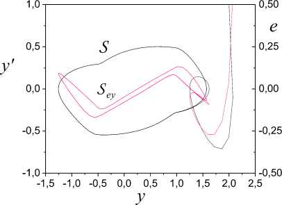
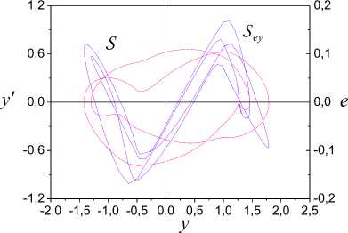
Solve the system (1) and obtain the set I . The phase portrait of the system (1) is showed in Fig.1.

Fig.1. Phase portrait of system (1)

We see that the framework S have features in points y_T =- 0.5 and y₂ = 1. Therefore, w_n = 1, w ₁₂ =- 0.5. We cannot make the decision on the form ^ ( y ) on the basis of the analysis S . Therefore, apply the design structural stage AO.

• F. Structural Stage of Design AO

Apply the approach proposed in the section III and construct the framework S . Synthesis S is based on application of the model (9). S is obtained on the time gap J_g = [ 10.4;31.4 ] s which corresponds to the system steady motion. The vector D in (9) is [ 0.06; 0.23; - 0.38 ] ^ . The framework S_ey is presented in Fig.1. We see what ^ ( y ) belongs to the class of nonlinearities with saturation.

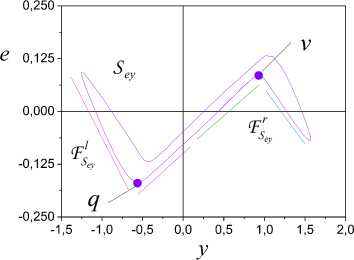
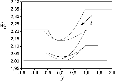
Fig.2. Framework S with the selected fragments

Estimate the system structural identifiability. It is determined with the possibility the identification of parameters ^ ( y ) . The analysis of the framework S shows that the system is h -identified. Estimate h -identifiability of the system.

Select in S fragments F ^l,F ^r (Fig. 2). They are marked with red and green straight lines in Fig. 2.

1,2

IH ^{r 0,8} IH ^l 0,4 0,0 -0

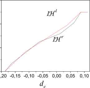
Fig.3. Cumulative frequency functions for fragments of framework S

The SI estimation is based on the structural-frequency approach described in the section III. Determine by frequency distribution functions H^l , H^r for fragments F^l,F^r . Obtain on the basis H^l , H^r cumulative frequency functions IH ^l , IH ^r (Fig. 3) and corresponding it the vectors L ( IH l ) , R ( IH^r ) . d_e is the pocket on e in Fig. 3.

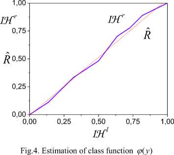
Model (11) has the form

RR = - 0.007 + 1.042 L ( IH¹ ) .          (48)

The determination coefficient of the model (48) is 0.992. Apply the statement 2 and estimate h -identifiability of the system. Show to estimation results of the SI in Fig. 4. The system has dimension D_h = 1. Therefore, ^ ( y ) belongs to single-valued function class.

Now determine by nonlinearity structural parameters. Apply the approach proposed in [22]. Consider the line sec tion of the framework S located between points q and v (Fig. 2). As parameter estimations in space (y,e) are not representative apply the following algorithm for finding of parameters.

Algorithm for the estimation of saturation parameters on the line section S .

ey

• 1.    Estimate h -identifiability of the system.

• 2.    Construct the framework S .

• 3.    Estimate the SI of the system. If the system is h -identifiable, then go to the step 4, otherwise the end of the algorithm.

• 4.    Go to S and allocate the bottom line section F .

• 5.    Calculate the coefficient of structural properties on F gv .

• 6.    Consider the section F + c F^ on which k_s ( t ) and e ( t ) have identical signs.

• 7.    Approximate the section F + c S^ the dependence

• 8.    Calculate the average e , k for e ( t ), k ( t ) on the time gap of definition F + .

• 9.    Determine by the estimation a + of true parameter a + as

  ~+ a j

  
  

  ea + k _s

  
  

ey

F (t) = a + + a+y (t), where a +, a+ are determined by means of LSM.

Apply this algorithm to the angle inclination estimation b_x ⁺ of the upper linear part S_e .

Algorithm application results:

• i)    lower line section: a+ = 0.18, w ₂ = 1.9;

• ii)    upper line section: b⁺ = 0.186 , i w₂ = 2.08.

So, we have for parameter w the area G = [ 1.9; 2.08 ] . As transition points in the saturation area are known, saturation levels ф (y ):

• 1)    if y_x =- 0.5 then ф (y ) e [ - 1; - 0.95];

• 2)    if y = 1 then ф (y ₂) e [1.9;2.08].

Average values in points y , y and obtain estimations: w _2г=- 0.975, w₂₂ = 1.99. The estimation for w is 1.99.

• H. Parametrical Stage of Design AO

The case 1 considered in section IV gives to model (8) and is well studied. Therefore, we will consider the case 2.

Let function ф ( y ) have the form (20). Apply for identification ф ( y ) the model

^W 2 w 11   if y >  w 11

^{ф (} y ) = ‘

^w 2 y  if y <  H ^ ,

/V /V      .p          ^

[ ^- w 2 w 1; if y <  w ;

where wˆ   wˆ  . Estimations for wˆ , wˆ  are obtained at the stage of structural synthesis.

The adaptive algorithm for tuning w ˆ has the form

-' / 2 ^ ya p if ( y ^e ( - 0.5;¹ ] ) &  ( w ₂ ⁶ G 22 ) ^ф                           ,           _x ,    (50)

0       if ( y 6 ( - 0.5;1 ] ) &  ( tv 2 e G 22 )

where y ₂ >  0 , (i_p e R is the adjusted coefficient of the model (23).

Structure choice of the algorithm (50) is directed to compensation not smoothness effect of the function ф ( y ).

The input r (t ) e PE_a has the form

r(t ) = 3sin ( 0.1 n t ) + sin ( 0.25 n t ) .           (51)

Fig.5. Frameworks S , S for system steady state with the input (50)

Remark 5. We applied different inputs at structural and parametrical stages. The input (51) ensures adaptation process with given quality indicators. The input (47) is constantly excited and allows identifying the function ф ( y ) . Frameworks S , S (Fig. 5) reflect the effect of the input (51) and show the transformation of frameworks presented in Fig. 1. The SI process is complicated and demands preliminary processing of the set I . The analysis S does not allow obtaining acceptable estimations for W , W . These results explain the current status of the design problem AO for nonlinear systems where the principle of linearization dominates.

Apply the method presented in section IV to the uncertainty estimation to in (23). The current estimation to is determined as

y d ( t ) - y d ( t^)if

ct( t) =

<

e ( t ) y ( t )

0        if

^{e (} t t) y ( t )

> 0.01

< 0.01

Structure choice of the algorithm for calculation a (t ) considers remarks made for the adaptive algorithm (50).

Adaptive model (23) has the form y = -ks + aуУ + alруРу + alР^рф + bp Pr + CT .    (53)

Apply algorithms (16), (18), (22), (27), (29), (49), (50), (52). Matrixes Г. for adaptive algorithms

Г = diag ( 0.015;0.0066 ) , Г = diag ( 0;0.05 ) ,

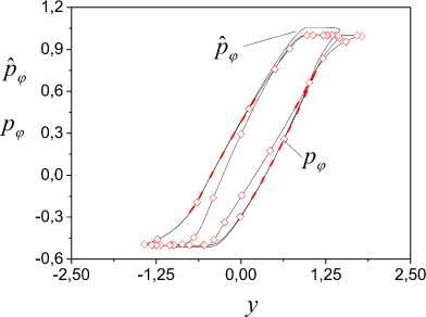
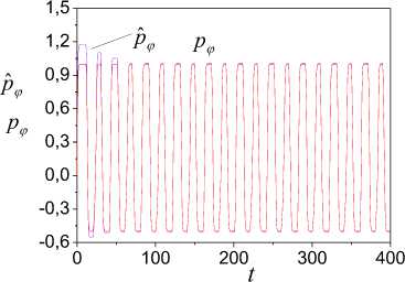
tification between pˆ and p . The determination coefficient for ^ is 0.999. This inference is confirmed with changes pˆ and p (Fig. 7). We do not show work results of the model (49) as they coincide with presented charts.

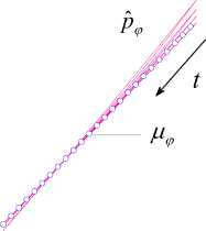
Fig.8. Frameworks reflecting tuning process of the variable pˆ

Frameworks showed in Fig. 8 give the better understanding of obtaining estimation accuracy for the variable p .

Г = diag ( 0;0.00375 ) , Г₂ = 0.03.

1,2

0,9

0,6

0,3

0,0

-0,3

-0,6

-1,0    -0,5     0,0     0,5     1,0     1,5

Р ф

Fig.6. Work adequacy estimation of the model (22)

Fig.7. Variation of variables pˆ  and p

Tuning results the AS _ф -system are shown in Fig. 6 -14. Fig. 6 - 8 represents the estimation process of the variable pˆ in two planes. Fig. 6 shows the adequacy estimation of the model (22) in the space ( р _ф , p _ф ) . We represent the linear secant ^ for the dependence iden-

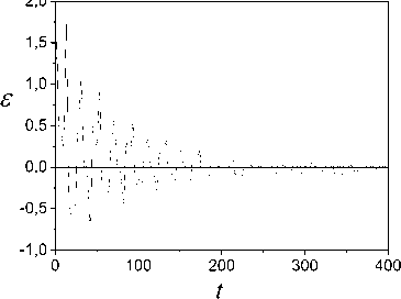
Fig.9. Error e of AO work

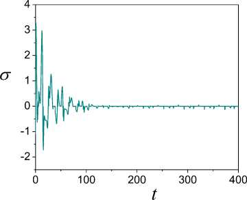
Change of the error e and the estimation of uncertainty ct are presented in Fig. 9, 10. Fig. 10 shows that the estimation accuracy to increases in the tuning process of AO.

Fig.10. Estimation ct the uncertainty to

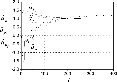
Parameters tuning of AO is shown in Fig. 11 - 14. Fig. 11 presents to the tuning of parameters aˆ , aˆ , b^ˆ  , and

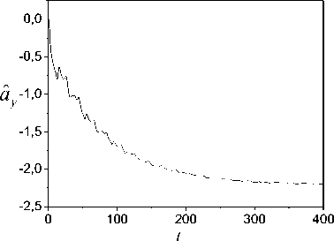
Fig. 12 shows tuning process a ˆ у . We see that tuning process finishes after 200 s.

Fig.11. Tuning of parameters a ˆ  , a ˆ  , b

Fig.12. Tuning of parameter a ˆ

Tuning of the parameter w ˆ of the model (49) on the application basis of the algorithm (50) is shown in Fig. 13, 14. Fig. 13 reflects of nonlinear processes effect in the adaptive system on the tuning w ˆ . We see that tuning process has a nonlinear character. This inference confirms Fig. 14.

Fig.13. Effect of the variable y on tuning of the parameter w ˆ

So, modelling results confirm the efficiency of the proposed approach to design of adaptive observers. Uncertainty influences on properties of AO. Tuning process increases:

• 1)    under interference of local parameters when basic parameters of AO are tunings;

• 2)    at the estimation of the nonlinearity and an unknown auxiliary p .

t

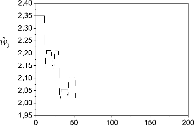
Fig.14. Tuning of parameter w ˆ

• VII. Conclusion

The method of adaptive observer design for nonlinear dynamic systems under uncertainty is proposed. It is based on the application of structural and parametrical approaches. The structural approach gives to identification problem solution for the nonlinear part of the system. It is based on the special class analysis of framework S . The decision about nonlinearity identifiability is to make on the basis S . We apply the sector sets method and structural-frequency approach to the estimation of the nonlinearity class. Parameter identification of the nonlinearity from the specified class is performed on the basis of the analysis S . The obtained structure and parameters of the nonlinearity are used at the parametrical design stage of AO.

We consider two cases of information use obtained at the structural stage. The first case corresponds the complete information about nonlinearity parameters. Algorithms for tuning of parameters AO are proposed and system identification stability is proved.

The second case is based on the assumption that the nonlinearity form is known (a result of the structural stage), and the set of nonlinearity parameters belongs to the specified area. The parametrized model for nonlinearity is proposed. The output of this model is the basis for the obtaining of current estimations of the auxiliary variable which is used in adaptive algorithms. This leads to the emergence of uncertainty in the adaptive system. The procedure is proposed for the estimation uncertainty. The adaptive system has the two-level structure. Interdependences between levels influence on the parameter tuning process the adaptive system. The stability of the adaptive system is proved. Modelling results of the adaptive observer are given.

Structural identifiability and the parametrical adaptation demand variables have property of the excitation constancy (EC). We show that the requirement of EC at considered development stages of AO differ. The parametrical stage demands the application of variables having the multifre quency form. The structural stage demands the analysis of variables have the single-frequency spectrum. Multifrequency complicates making decision on the nonlinearity class. Explain this with the fact that the nonlinear dynamic system reacts to each harmonic of the input. Multi-frequency complicates framework S (see Fig. 5) and activate the appearance of fragments which insignificant framework give. Solutions of this problem are known and we will consider them in the following publication.

• Appendix A.    Proof of Theorem 4

Consider Lyapunov function V ( t ) (31). V ( t )on motions AS -system has the form

V = - kE² + V_K - V_K < - 2 kV .      (A.1)

K    K         E

Apply the condition 1) theorem 4. As V(t) < 0 the system AS is stable. Integrate V(t) on time and obtain

t

• V ( 1 0 ) - 2 k J V e ( r )d r >  V ( t ).

t ₀

As V ( e , A K ) satisfies the condition 1) theorem 4, all trajectories of the system AS lie in the area G_z = { ( e , A K ) : V(t ) <  V ( t ₀) } . We have the estimation for the AS - system

t

J 2 kV E ( r ) d r <  V ( t о )- V ( t ).

t ₀

• Appendix B.    Proof of Lemma 1

Write V ( t )

V =-kE2 + eAKtP <-kE2 + El |AKTP|.

Apply the inequalities (33) and [31]

• - az2 + bz < —az— + — ,(B.2)

22a where a > 0, b > 0, z > 0 . Present (B.1) as

V = -kE2 + eAKP < -kE2 + |e| | aktp| < к 2 i т               «в (r)

— E2 + — aktbpak < -kV + l()

• 2     2 k      P         E     k

So, we obtain M ⁺ -property for V from (B.3).

Appendix C. Proof of Lemma 2

Write V ( t )

VK (t) = -eAKtP .(C.1)

where O = {0, 0³ m } c R x R ^{3 m} x J _Om is the system equilibrium position, O ( O ) is some neighbourhood of the point O , 0^{3 m} g R ^{3 m} is the zero vector, 3 >  0 is a some number, t ^{g [0,} / I = J 0, „ .

Apply (C.2) and present (C.1) as

V_K ( t ) = - 3 ( a k^tb a k + e ² ) = - ³ &ak^tb ak - b(|e |+Va k^tb a k V +

(C.3)

3|e| V a k^tb a k <

— Я А К В A K + 3 e Va k^tb a k .

Apply to (C.3) inequalities (B.2), (33) and obtain

V_K ( t ) <-- 3 A K^TB a k + 3| e| A kk^t aa k <

— 3 A K^TB a k + - 3e ²<           (C.4)

• 3         , .        8

• - - Зав . ( Г ) V k + з 8 V e .

So, M ⁺ -property for V_K has the form

Vk <-- Зав1 (Г) Vk + - 3Ve .

• Appendix D. Proof of Theorem 6

The proof of the theorem 6 matches the proof of the theorem 4. It is based on the use of the Lyapunov function (31). Trajectories AS -systems according to the theorem 4 are limited and lie in the area G_z = { ( e , A K ) : V(t ) <  V ( t ₀) } . As P is limited and depends on P ^ˆ , therefore, also the vector P ^ˆ is limited.