Study of Memory Effect in a Fuzzy EOQ Model with No Shortage

Published Online November 2019 in MECS

For a real situation of the business, market changes rapidly. Due to the fact, some parameters and variables are highly uncertain. In such situations, these parameters and variables are described as fuzzy parameters. The fuzzification declares authenticity to the model by allowing vagueness in the whole cost parameters which brings it closer to reality. We want to generalize the concept of the paper D.Sharmita etal [18] using fractional calculus on the basic EOQ model. Here, fractional calculus has been applied instead of ordinary calculus. Fractional order derivative and fractional order integration is used to include non-locality of the system. Fractional calculus are becoming a favourite research topic to the different field researchers.

Recently, the application of fractional order integration and differentiation becomes a hot research topic. Fractional integration and fractional differentiation are generalizations of notions of integer-order integration and differentiation and it can include n-th derivatives and n-fold integrals. Physical interpretations of any mathematical theory can close to reality and help to connect to the real world problem. Fractional calculus has some advantage from the ordinary calculus. For example, some properties of fractional order derivative can include the violation of Leibnitz rule and violation of chain rule. Some unusual properties [21] of the fractional order derivatives describe complex properties of the chain rules. The physical interpretation of the fractional calculus is that fractional order of fractional derivative and integration is an index of memory [1,9,10,11]. Using the concept of memory several research papers have been developed [1,2,3,4,5,6,7]. Some of them are discussed shortly. Application of memory effect using fractional calculus was done by M.Saedianetal[1] in the biological model. Besides, Tarasovaetal[2,3,4,5,6,7] have developed many research article using the concept of memory effect to the economic models. Memory dependent inventory models [9,10,11,23,24,20] have been developed by Pakhira et al to establish memory effect in EOQ models with different terms and conditions. Different     memory      dependent      inventory models[9,10,11,23,24,20] have been developed in different articles without fuzzy environment.

Due to the above fact, we want to incorporate here fuzzy environment. In this paper, our aim is to develop a memory dependent EOQ model under the fuzzy environment using fractional calculus. Some researchers have worked on the Classical inventory model [17,18] under the fuzzy environment with assuming different conditions on the cost parameters. Some of them are discussed shortly. As for example, Majumdar.P etal [17] developed an EPQ model of deteriorating items under partial trade credit financing and demand declining market in crisp and fuzzy environment. N.K.Mandal[18] developed a Fuzzy economic order quantity model with ranking fuzzy cost parameters. D. Sharmita etal [18] established an inventory model for deteriorating items with shortages and exponential demand involving fuzzy environment. Besides, Dutta.D et al also developed a fuzzy inventory model for deteriorating items with shortages under fully backlogged condition. Different above mentioned authors do not use the beauty of fractional calculus in their model. Fractional has a beautiful property.

In this paper, this analogy ’fractional order as the index of memory’ has been used to illustrate the model. Fractional order inventory model has been developed to include memory effect under the fuzzy environment. The fractional order model is also fuzzified using Graded mean integration method and signed distance method. Since the fuzzy environment can close to reality with incorporating uncertainty behavior to the system. Inventory level with respect to time has been drawn to show the changing behavior for (i) long memory,(ii)short memory,(iii) memory less system. Then we want to discuss the rearrangement part of the paper to overview easily.

The rest of the paper is organized as follows: In section III, the preliminary introduction of fractional calculus are introduced. Section IV (C )is about the formulation of the classical inventory model. In section V, we have discussed the procedure of fractionalization of the classical model. In section VI, Mathematical formulation of the fractional order inventory model is discussed. Fuzzy fractional order inventory model has been given in the section-VII, Numerical examples in the section-VIII, Graphical presentations are done in the section-IX. Lastly, conclusions and future research works are discussed in the section-X.

• II.    Related Developed Work

The classical fuzzy inventory model has been described in the paper[18,22].This paper is followed from this two papers[18,22].The Memory concept has been followed from the different papers like[10,11,20,21,23,24].

• III.    Review of Fractional Calculus

To develop the model, Caputo fractional order derivative and fractional Laplace transform method has been used, are discussed shortly.

• A.    Euler Gamma Function

  Euler’s gamma function is one of the best tools in fractional calculus which was proposed by the Swiss mathematicians Leonhard Euler (1707-1783).The gamma function Г ( x ) is continuous extension from the factorial notation. The gamma function is denoted and defined by the formulae

to

Г ( x ) = j t ^{( x - 1)} e ^- dt     x >  0           (1)

Г ( x ) is extended for all real and complex numbers and the gamma function satisfies some basic properties

Г ( x + 1) = x Г ( x ) ^ Г ( x ) = ^⁽ x ⁺ ^

x

=    , г|- 7

2 I 6

Numerically x ! can be evaluated for all positive integer values numerically but Г ( x + 1) can be evaluated for real values.

• B.    Riemann-Liouville fractional derivative(R-L)

Left Riemann-Liouville fractional derivative[12-13] of order a is denoted and defined as follows

d : ( f ( x )) =

m

I d 1

Г ( m - a ) ( dx J

x j (x - T )(m-a-1) f (T ) dT

a

where x >  0

Right Riemann-Liouville fractional derivative of order a is defined as follows

D ( f ( x )) =

Г ( m - a )

mb

I- d | J( T - x )^{( m -a - 1)} f ( T ) d T

I dx J                        (4)

x where x > 0

Riemann-Liouville fractional derivative of any constant function is not equal to zero which creates a distance between ordinary calculus and fractional calculus.

• C.    Caputo fractional order derivative

Left Caputo fractional derivative [14] for the function f ( x ) which has continuous, bounded derivatives in

[ a , b ] is denoted and defined as follows

x

C D : ( f ( X )) = -------- J ( X - T ) ⁽ m - ^а - 1) f m ( t ) d T

Г ( m - а ) а                       (5)

where 0 <  m - 1 <  а <  m

Right Caputo fractional derivative for the function f ( x ) which has continuous and bounded derivatives in

[ a , b ] , is defined as follows

b cd: (f ( X)) = --------- J (T - X)(m -а-1) fm (T ) dT

Г(m - а) X where 0 < m -1 < а < m cd: (A) = 0, where A = constant.

• D.    Fractional Laplace transforms Method

The Laplace transform of the function f(t) is defined as to

F ( s ) = L ( f ( t )) = J e ^{- st}f ( t ) dt            (7)

where s>0 and s is called the transform parameter. The Laplace transformation of nth order derivative is defined as n-1

L ( f n ( t )) = sⁿF ( s ) - ^ s n ^- k ^{- 1} f k (0)         (8)

k = 0

where fn (t) denotes nth derivative of the function f with respect to t and for non – integer m it is defined in generalized form[8-9] as, n-1

L ( f m ( t )) = s^mF ( s ) - £ ff " ^{- k - 1}(0)        (9)

к = 0

Where, ( n - 1) <  m <  n .

In the next sections, we first discuss the classical inventory model which can help to provide a link to establish the fractional order inventory model.

• IV. Classical Inventory Model

The classical model has been developed in this section.

• A.    Notations

The notations are given to develop the inventory model.

Table 1. Different symbols and items for the model.

( i ) D ( t ) : Demand rate	( ii ) Q : Total order quantity
( iii ) U : Per unit cost	( iv ) C : Inventory holding cost per unit
( v ) C : Ordering cost or setup cost	( vi ) I ( t ) : Stock level or inventory level
( vii ) T : Ordering interval	( viii ) HC a , в : Inventory holding cost per cycle for the fractional order inventory model
( ix ) TG * : Optimal ordering interval using Graded Mean integration method	( x ) tc : vg :T °tal average cost using graded mean integration method.
( xi ) TS : Optimal ordering interval for signed distance method	( xii )( B ,.),( Г ,.): Beta function and gamma function respectively
( xiii ) TCS * : Minimized total average cost during the total time interval [0, T ] using signed distance method	( xiv ) TCG : Minimized total average cost during the total time interval [0, T ] using graded mean integration method
( xv ) TCavS : Total average cost during the total time interval using signed distance integration method

Next, we want to discuss the assuming some assumptions to develop the model.

• B.    Assumptions

The below assumptions are made to develop the model. (i) Lead time is zero,(ii)Time horizon is infinite,(iii)There is no shortage,(iv)There is no deterioration.(v) Demand rate is D ( t ) = ( a + bt ) for 0 <  t <  T . Then, we have discussed the classical inventory model formulation.

• C.    Classical inventory model Formulation

During the total period [0, T ] , the inventory level depletes due to the demand rate ( a + bt ), a , b >  0 where the shortage is not allowed. Hence, the classical model is governed in by the ordinary differential equation as

d ⁽ I ⁽ t )) = - ( a + bt ) for 0 <  t <  T        (10)

dt with boundary conditions are I(t) = 0 and I(0) = Q .

Inventory level is obtained by solving (10) with the boundary condition I ( t ) = 0 in the following form

I ( t ) = a(T - 1 ) + b ( T ² - 1 ²)             (11)

Using initial condition I (0) = Q , the optimal order quantityis obtained as,

Q =

aT + bT²

Corresponding total inventory holding cost over the time interval [0,T] is denoted by HC ( T ) and defined as follows

T

HC(T) = C JI a(T-t) 0 V

+ 2 ( ^T - - t ² fy

C is the holding cost per unit.

Hence, the total cost is as

TC ( T ) = Purchasing cost ( PC ) +holding cost( HC ( T ) +set up cost ( C )

лTC(T)

aT + bT

Therefore, the total average cost per unit time per cycle is

in which k ( t - t ') plays the role of a time-dependent kernel. For Markov process it is equal to the delta function < ? ( t - 1 ')that generates the equation (10).In fact, any arbitrary function can be replaced by a sum of delta functions, thereby leading to a given type of time correlations. This type of kernel promises the existence of scaling features as it is often intrinsic in most natural phenomena. Thus, to generate the fractional order model we consider k ( t - 1 ') =-------- ( t - 1 ') “ ^{- 2} , where

Г (1 - a )

d ( t ) = - о D . ^{- 1 )}( a + bt )             (18)

Now, applying fractional Caputo derivative of order ( a - 1) on both sides of (18), and using the fact that Caputo fractional order derivative and fractional integral are inverse operators, the following fractional differential equations can be obtained for the model

C D ( I ( t ) ) = - ( a + bt ) or equivalently

TOC ” ( T )

d ^a ( I(t) ) dt ^a

- (a + bt) ,

T

Thus, the objective of the classical EOQ model can be represented in the form as,

f        , _x  JUQ + HC ( T ) + C)

₍ MinTC ( T ) = CQ ^(—--

Subject to T >  0

In the next section, we have developed the fractional order model with memory kernel.

V. Fractional Order Inventory Model with Memory Kernel

To study the influence of memory effects, first the differential equation (10) is written using the memory kernel function in the following form [1].

dI ( t ) = - J k ( t - t ' ) ( a + bt ')dt '          (17)

for 0 <  a <  1.0, 0 <  t <  T

with boundary conditions I(T ) = 0 and I (0) = Q .

Depending on the range of _a , long memory effect and short memory effect has been defined.

Long and Short Memory Effect: The strength of memory depends by the order of the fractional order derivative and fractional order integration. If the fractional order index a is in (0,0.5] then we define the system as the long memory affected system and for short memory effected system a is in (0.5,1].

In the next section mathematical solution and analytical results are discussed due to reach the final numerical result.

VI. Mathematical Formulation of the Fractional Order Inventory Model

Here, we consider the fractional order inventory model which will be solved by using Laplace transform method with the boundary condition I(T ) = 0. In operator form the fractional differential equation of (19) can be represented as

Da (I(t)) = -(a + bt)

d “(20)

D ^a = — ,with I ( T ) = 0

dtav

Therefore, the total average cost per unit time per cycle is,

where the operator D ^a stands for the Caputo fractional order derivative with the operator

_av _( UQ 1 HC _a , p ( T ) 1 C 3 )

TC a , p

T

( d * = cd : ).

Solving the above equation (20), we get the required inventory level with fractional effect

I ( t )

' a ( T ’ - 1 " )    b ( T " * 1 - 1 " ^{1 1} )'

Г (1 + a )       r ( a + 2 )

'    C 1 b   '     1 __ B ( a 1 2, p ) ' _T„ 1 p

Г ( a 1 2 ) Vr ( p 1 1 ) Г ( p ) J

₊    C i a   '     1 __ B ( a 1 1, p ) ' _t* 1 p - 1

r ( a 1 1 ) (г ( p 1 1 ) Г ( p ) ^J

1 z ^aU . T ^{a - 1} 1 z ^bU , T ^a 1 CT ¹

Г ( a 1 1 )        Г ( a 1 2 )        ³

The inventory model can be written as follows

For a = 1.0, the equation (21) becomes to the equation (11).

Using the boundary condition I(T ) = 0 on the equation (21), the total order quantity is obtained as

' AT ^{a - 1} 1 BT ^a 1 CT ^{a 1 p - 1} '

MinTCav = I           1               I ap  V1 DTa 1 p 1ET-1       J A (26)

Subject to T >  0

¹ ( 0 ) = Q =

' ^a ( T ^a )

Г (1 + a )

V

b ( T ^{1 1 a} ) ' * ^r ( a + ² ) ,

and corresponding the inventory level at time t being,

¹ ( t )

' a ( T " - 1 " )    b ( T - ^{1 1} - 1* ^{1 1} )'

Г (1 + a )       r ( a + 2 )

-^^.B. =

r ( a 1 1 )   ¹    r ( a 1 2 )

Ca '    1     _ B ( a 1 1, p ) '

r ( a 1 1 ) Vr ( p 1 1 )      Г ( p ) ^J

C 1 b   '     1 ^B ( a 1 2, p ) '

r ( a 1 2 ) (r ( p 1 1 )      Г ( p )   ^J ,      ³

Next, we have discussed the fuzzyfication of the fractional order inventory model

Purchasing cost is as

' a ( T ^a )     b ( T ^{1+ a} ) '

PC = U X Q = U — —-1—7---'-     (24)

Г (1 + a ) r ( a + 2 )

(where U is the per unit cost)

For the model (19), the p-(0 < p < 1) order total inventory holding cost is denoted as HCa p (T) and defined as

• VII.    Fuzzified of Fractional Order Inventory Model

The fuzzyfication is followed from [22].The related fuzzy inventory model(classical) is described in[18,22].

Here, we fuzzify the cost parameters per unit cost ( U ) , holding cost ( C ) ,setup cost ( C ₃) as follows

U = ( a 1 , b 1 , c 1 ) , C 1 = ( a ₂, b ₂, c ₂ ) , C ₃ = ( a ₃, b ₃, c ₃ )

HC _a , p ( T ) = C 10 D T ^{- p} ( I ( t ) )

T

= f T - 1 У ^{p - 1 )} UUM r ( p ) J ⁽     )    ⁽⁽⁾⁾

av

TC a , p

( UQ 1 HC a , p ( T ) 1 C 3 )

T

CaT ^{( a 1 p} ) '     1     _ B ( a + 1, в ) '    (25)

r ( a 1 1 ) Vr ( p 1 1 ) Г ( p )    ,

CbT ^{a 1 p}  '    1      B ( a 1 2, p f

¹ Г ( a 1 2 ) Vr ( p 1 1 ) Г ( p )    ,

' ( a 2 , ^b 2 , ^c 2 ) ^b '     1     _ B ( ^{a 1} 2, ^p ) ' _Ta 1 p

r ( a 1 2 ) Vr ( p 1 1 )      Г ( p ) ^J

₊ ( a 2 , ^b 2 , ^C 2 ) a '     1     _ ^B ( « ¹ 1, ^p ) ' .pa 1 p

r ( a 1 1 ) Vr ( p 1 1 )      Г ( p ) ^J

₊ a ( a 1 , ^b 1 , ^C 1 ) -pa - 1 ₊

Г ( a 1 1 )

( p is considered as integral memory index)

b ( a , b , c )

_V r ( a 1 2 )

t * 1 ( a ₃, b , c ₃) t ⁴

Г ( a 2 ) b Г     1     _ B ( a + 2, в ) ) Ta + в   ' r ( a + 2 ) (r ( в + 1 )      Г ( в )    J + ( a 2 ) a Г    1     _ Вк а+ ^. РХ ) Ta + в -1 r ( a + 1 ) (r ( в + 1 )      Г ( в )    J a(a,)       ,      b(aA     „   , х    , + — '     T a - 1 + —11 T a + ( a, ) T -1 r ( a + 1 )        r ( a + 2 )      v 37 Г   ( b 2 ) b Г     1       B ( a + 2, в ) ) Ta + в   )

r ( a + 2 ) (r ( в + 1 )      Г ( в )    J + ( b 2 ) a Г     1       B ( a + 1, в ) ) ya + в -1 r ( a + 1 ) (r ( в + 1 )      Г ( в )    J +   a ( b 1 ) T a - 1 +   b ( b 1 )  T a + ( b ) T -1 r ( a + 1 )        r ( a + 2 )      v 3/ Г ( c 2 ) b Г     1       B ( a + 2, в ) ) Ta + в   )

r ( a + 2 ) (r ( в + 1 )      Г ( в )    J + ( c 2 ) a Г    1     _ В^О + Х 1Р1 ) Ta + в -1 r ( a + 1 ) (r ( в + 1 )      Г ( в )    J +   a ( c 1 )  t a - 1 +   b ( c 1 ) x t a + ( c ) t r ( a + 1 )        r ( a + 2 )      v 37

• A.    Signed distance method

Next, we have discussed the signed distance method its corresponding inventory model.

Fractional order inventory model has been defuzzified using signed distance method[22].

Using signed distance method total average cost is written as follows

U   ( a l , ^b 1 , c l ) , C 1    ( a 2 , b 2 , c 2 ) , C 3     ( a 3 , b 3 , c 3 )

TC aSS = 1 ( TC + 2 TC ₂ + TC )

' b ( a 2 + 2 b 2 + c 2 ) Г 1       B ( a + 2, в ) ) _r+ в

4 Г ( а + 2 )    (r ( в + 1 )      Г ( в ) ^J

_TCavS ₌  , a ( a 2 ^{+ 2} b 2 ⁺ c 2 ) Г 1       ^B ( “ ^{+ 1, в} ) ) _Ta + в - 1

^a • ^в         4 Г ( а + 1 )    (r ( в + 1 ) Г ( в ) ^J

+ a (a + 2b + c) Ta-1 , b (a + 2b + c ) Ta , (a3 + 2b3 + c3

4Г(а +1)           4Г(а + 2)

In this case,Inventory model can be written as follows

- Г ATa-1 + BTa + CT Min TCavS = I

'   (+ DT ^{a + в} + ET ^{- 1}

Subject to T >  0

a ( a + 2 b + c )      b ( a , + 2 b + c )

=   4Г(а +1)   ’ 1 =   4Г(а + 2)

a ( a ₂ + 2 b ₂ + c ₂ ) Г    1       B ( a + 1, в ) )

C =   4Г(а +1)   (г( в +1)     Г( в)

b ( a ₂ + 2 b ₂ + c ₂ ) Г   1       B ( a + 2, в ) )      ( a ₃ + 2 b + c )

=   4Г(а + 2)  (r( в +1)     Г(в)   J,  =

• B.    Graded mean integration method

Fractional order inventory model has been defuzzified using graded mean integration method[22].

Using graded mean integration method, total average cost is written as follows

U   ( a1 , b1, c1 ) , C1    ( a 2 , b2 , c 2 ) , C3    ( a 3 , b3 , c3

TCavc = 1 (TCav + 4TCav  + TCav)

a , в        6 \       a , в 1                a , в ,2             a , в ,3 /

^Г b ( a 2 + 4 b 2 + c 2 ) Г 1       ^B ( ^{a +} 2, ^в ) ) _т„ + в

6r(a + 2)   (r( в +1)     Г( в)

₊ a ( a 2 ^{+ 4 b} 2 ⁺ c 2 ) Г     1       ^B ( ^{a + 1 в} ) ) _Г + в - 1

6 r ( a + 1 )    (r ( в + 1 )      Г ( в ) ^J

+ a (a1 + 4b1 + c1 ) T„-1 j b (a1 + 4b1 + c1 ) T„ j (a3 + 4b3 + c3

6r(a + 1)           6r(a + 2)

In this case,Inventory model can be written as follows

Min TC avG

J               a , в

AT ^{a - 1} + BT ^a + CT + DT ^{a + в} + ET ^{- 1}

Subject to T >  0

a ( ^a 1 ^{+ 4} b , ^{+ c} 1 )        ^b ( a , ^{+ 4} b , ^{+ c} 1 )

a =-----;----;—, b, =----------—,

6 r ( a + 1 )      ¹      6 r ( a + 2 )

a ( a ₂ + 4 b + c ₂ ) Г     1       B ( a + 1, в )

=    6 r ( a + 1 )    [г ( в + 1 )      Г ( в )

b ( a ₂ + 4 b + c ₂ ) Г    1       B ( a + 2, в ))g  ( ^й з + 4 Ь з + С з )

=    6 r ( a + 2 )    [г ( в + 1 )      Г ( в ) J ,   =       6

• VIII.    Numerical Example

To illustrate numerically of the developed fractional order inventory model, we consider empirical values of the various parameters in proper units as Y = 45, ( a ! , b_x, c_x ) = ( 12,14,16 ) ,

( a ₂, b ₂, c ₂ ) = ( 19,20,24 ) , ( a ₃, b ₃, c ₃ ) = ( 280,300,310 ) an required solution has been made using matlab minimization method.

where

• A.    Optimal ordering interval and Minimized total average cost using signed distance method.

Table 2. Optimal ordering interval and minimized total average cost using signed distance method where 0 <  a < 1.0, в = 1.0 described in sectionVII.

a	в	* s Ta , в	tc « * в
0.1	1.0	1.6811	1.4979x103
0.2	1.0	1.4845	1.6404x103
0.3 (growing memory effect)	1.0	1.3033	1.7508x103
0.4	1.0	1.1396	1.8238x103
0.5	1.0	0.9952	1.8570x103(max imum)
0.6	1.0	0.8722	1.8518x103
0.7	1.0	0.7714	1.8129x103
0.8↑	1.0	0.6927	1.7480x103
0.9	1.0	0.6341	1.6653x103
1.0	1.0	0.5927	1.5731x103

From table 2, it is found that for a = 0.5 minimized total average cost is maximum then gradually falls down. Hence, suddenly, business policy falls down then gradually improves. In general, in reality it happens always i.e. profit increase or decrease with respect to its previous effect.

Table 3. Optimal ordering interval and minimized total average cost using signed distance method for 0 <  в <  1.0, a = 1.0 described in section-VII-A.

Ct	в	* s Ta , в	tc « * в
1.0	0.1	1.15339(maximum)	1.2231x103
1.0	0.2	1.0112	1.3404x103
1.0	0.3	0.8928	1.4341x103
1.0	0.4	0.8007	1.5035x103
1.0	0.5	0.7318	1.5505x103
1.0	0.6	0.6814	1.5788x103
1.0	0.7	0.6454	1.5918x103
1.0	0.8 ↑	0.6202	1.5934x103(maximum)
1.0	0.9	0.6033	1.5836x103
1.0	1.0	0.5927	1.5731x103

From table-3, it is clear that in absence of differential memory index in presence of integral memory index, minimized total average cost is maximum at в = 0-8 then gradually falls down above and below. Hence, suddenly, business policy falls down then gradually improves. In absence of differential memory index, minimized total average cost is low compared to the presence of differential memory index.

Table 4 shows that in presence of integral memory index with varying differential memory index, minimized total average cost is very much low compared to the two cases (i) presence of integral memory index in absence of differential memory index,(ii) presence of differential memory index in absence of integral memory index.

Table 4. Ta s* _в and TC^s _a * _в using signed distance method where 0 <  a < 1.0, в = 0.5 described in section-VII-A.

Ct	в	* s T a , в	TC s *, в
0.1	0.5	3.5443	1.1330x103
0.2	0.5	2.8779	1.2873x103
0.3	0.5	2.3685	1.4256x103
0.4	0.5	1.9601	1.5406x103
0.5	0.5	1.6251	1.6256x103
0.6	0.5	1.3495	1.6757x103
0.7	0.5	1.1267	1.6893x103(maximum)
0.8↑(growing memory effect)	0.5	0.9529	1.6686x103
0.9	0.5	0.8235	1.6196x103
1.0	0.5	0.7318	1.5505x103

From the above table 2-4 where minimized total average cost and optimal ordering interval are evaluated using signed distance method, the conclusions are done as

• (i)    In presence of differential memory index in absence of integral memory index, for a = 0.5 minimized total average cost is maximum then gradually falls down. Hence, suddenly, business policy falls down then gradually improves.

• (ii)    In absence of differential memory index with presence of integral memory index, minimized total average cost is maximum at в = 0.8 then gradually falls down above and below. Hence, suddenly, business policy falls down then gradually improves. In absence of differential memory index, minimized total average cost is low compared to the presence of differential memory index.

• (iii)    In presence of integral memory index with varying differential memory index,minimized total average cost is very much low compared to the two cases (i) presence of integral memory index with absence of differential memory index,(ii) presence of differential memory index with absence of integral memory index.

• B.    Optimal ordering interval and minimized total average cost using graded mean integration method

Table 5. Optimal ordering interval and minimized total average cost using graded mean integration method where 0 <  a <  1, в = 1.0.

a	в	G * T a , в	TC G . p
0.1	1.0	1.6917	1.4917x103
0.2	1.0	1.4937	1.6338x103
0.3 (growing memory effect)	1.0	1.3114	1.744x103
0.4	1.0	1.1466	1.8171x103
0 .5	1.0	1.0014	1.8508x103(maxi mum)
0.6	1.0	0.8776	1.8462x103
0.7	1.0	0.7762	1.8081x103
0.8↑	1.0	0.6969	1.7439x103
0.9	1.0	0.6378	1.6620x103
1.0	1.0	0.5960	1.5704x103

From table 5 , table 2 , it is observed that minimized total average cost using graded integration method is low compared to the signed distance method.Table-5 also shows that at α = 0.5 , minimized total average cost becomes maximum then gradually decreases below and above. Profit once, loses then gradually increases below and above. Optimal ordering interval gradually increases with respect to memory index.

to favorable or unfavorable social, environment, cost parameters are highly uncertain. To eradicate this uncertainty, fuzzy cost parameters are incorporated.

In the next section, we have discussed the pictorial behavior of the total average cost function with respect to different memory indexes and inventory level, inventory holding cost for different memory index with respect to time.

Table 6. T _α ^G _{, β} ^* and TC _α ^G _, ^* _β using graded mean integration method where 0 <  β ≤ 1.0, α = 1.0 described in section-VII.

α	β	G * T α , β	TC α G , * β
1.0	0.1	1.1564	1.2222x103
1.0	0.2	1.0151	1.3384x103
1.0	0.3	0.8970	1.4312x103
1.0	0.4	0.8050	1.5001x103
1.0	0.5	0.7359	1.5470x103
1.0	0.6	0.6854	1.5752x103
1.0	0.7	0.6491	1.5884x103
1.0	0.8↑(growing memory effect)	0.6237	1.5902x103(maximum)
1.0	0.9	0.6067	1.5834x103
1.0	1.0	0.5960	1.5704x103

From table 6, table 3, it is clear that numerical value of the minimized total average cost using graded integration method is low compared to the signed distance method.

Table 7. T _α ^G _{, β} ^* and TC _α ^G _, ^* _β using graded mean integration method where 0 <  α ≤ 1, β = 0.5 described in section-VII.

α	β	G * T α , β	TC α G , * β
0.1	0.5	3.5708	1.1277x103
0.2	0.5	2.8972	1.2816x103
0.3	0.5	2.3832	1.4196x103
0.4	0.5	1.9718	1.5344x103
0.5	0.5	1.6346	1.6194x103
0.6	0.5	1.3574	1.6698x103
0.7	0.5	1.1333	1.6839x103
0.8↑(growing memory effect)	0.5	0.9585	1.6637x103
0.9	0.5	0.8283	1.6154x103
1.0	0.5	0.7359	1.5470x103

From table 7 and 4, it is found that numerical values of the minimized total average cost using graded integration method is low compared to the signed distance method.

From all observations of the numerical examples, it is observed that numerical values of the minimized total average cost using graded integration method is low compared to the signed distance method.

Here, we want to include a real world example where, this mathematical results can knock. All numerical examples clear that at once profit is losses then gradually increases. In reality, in the village- area, selling rate of shoes, cosmetic products, clothes increase in the season wise in the different festivals of the local area. For that reason, profit of the business increases or decreases. Due

• IX.    Graphical Presentations

Scatter diagram of the minimized total average cost and optimal ordering interval using the above tables.

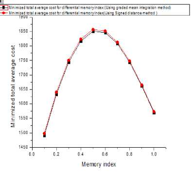
Fig.1. Comparison of the minimized total average cost with respect to differential memory index using (i) graded mean integration method (ii) signed distance method.

From fig.1, it is clear that the graph of the minimized total average cost is parabolic type whose vertex is upward. On the other hand, it is also clear that, the numerical values using graded mean integration method is low compared to the signed distance method.

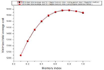
Fig.2. Comparison of the minimized total average cost with respect to Integral memory index corresponding (i) graded mean integration method (ii) signed distance method.

From fig.2, it is found that the minimized total average cost function is not exactly parabolic but approximately. On the other hand, it is also clear that, the numerical values using graded mean integration method is low compared to the signed distance method but their difference is very negligible.

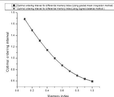
Fig.3. Comparison of the Optimal ordering interval with respect to differential memory index (i) graded mean integration method (ii) signed distance method.

From fig.3, it is found that the minimized total average cost function is exponential type. On the other hand, it is also clear that, the numerical values of the optimal ordering interval using graded mean integration method is high compared to the signed distance method but their difference is very negligible.

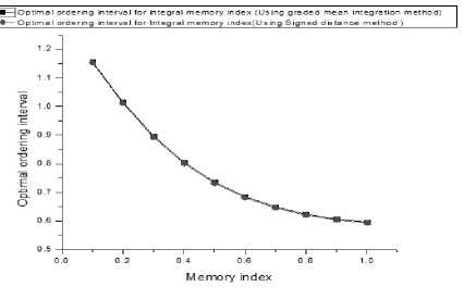
Fig.4. Comparison of the optimal ordering interval with respect to Integral memory index corresponding (i) graded mean integration method (ii) signed distance method respectively.

From fig.3&4, it is observed that the minimized total average cost is exponential type. But the numerical values of the optimal ordering interval for presence of differential memory index is high compared to the absence of differential memory index i.e. in presence of integral memory index.

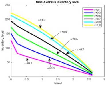
Fig.5. Time-t versus Inventory level for different values of α .

From fig.5, it is clear that qualitatively different behavior of inventory level is found for(i) long memory effect,(ii) short memory effect,(iii) memory less system. Rate of change of inventory level for long memory effect is concave type but in short memory effect, is not concave type.

(a)

(b)

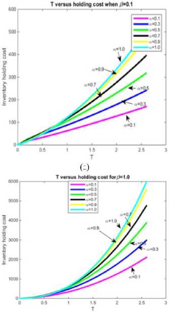
Fig.6. (a-b)Inventory holding cost versus ordering interval- T for different values of α , β .

From fig.6.( a - b ), it is observed that for gradually increasing memory effect(here, memory effect quantity α ) holding cost is gradually decreasing for different values of β . From the fig.6, it is observed that initially lowest inventory holding cost is at α = 0.1 then gradually increases highest inventory holding cost is at α = 0.1 .

500 0

T versus total average cost using signed distance method for β=0.1

α=0.1

α=0.7

α=0.9

α=1.0

0.5           1           1.5           2           2.5           3

Ordering interval-T

(a)

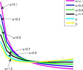
Fig.7. (a)ordering interval- T- Total average cost using signed distance method for different values of α , β .

From the fig.7.(a) we can conclude that total average cost using signed distance method is concave type. Total average cost lowest at the a = 0.1 with respect to ordering interval as well as total average cost reaches highest level for lowest ordering interval at a = 0.1.

(a)

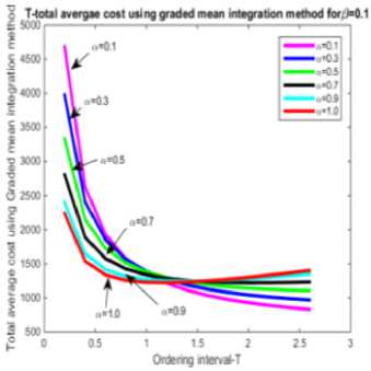
Fig.8. (a)Ordering interval- T - total average cost using graded mean integration method for different values of a , Д

In fig-8(a), we want to show the behavior of total average cost function with respect to the ordering interval for different memory index.

From all fig.8.(a)it is observed that total average cost becomes low for a = 0.1.

• X.    Conclusion

In this paper, some useful ideas were presented to deal with fractional order inventory model with fuzzy environment. In economic model memory effect should be incorporated due to the fact that some economic facts depend on the past experience such as environment, social situation, product quality can increase or decrease the selling rate of the product. Fuzzyfied can close to the reality to incorporate the uncertainty behavior of some economic parameters like set up cost, holding cost, per unit cost. We have also analyzed the fractional order inventory model under fuzzy environment to evaluate the optimum results of ordering interval and total average cost.Fig.5, 6,8helps to conclude that the neglect of memory effects in the economic model may lead to qualitatively different output of inventory leveland holding cost, minimized total average cost.Numerical examples provide us that minimized total average cost using graded integration method is low compared to the signed distance method. In long memory effect profit is maximum compared to the low memory effect as well as memory less system for both methods (i) graded mean integration method,(ii) signed distance method. This paper helps to come out the developed thought of classical fuzzy inventory model. This paper also helps to include reality of the system using the memory effect property of the system. More work on the inventory system can be done under the fuzzy environment using fractional calculus for the future research work.

Acknowledgements

Authors would like to express their sincere thanks to the referees and editors for their valuable comments and suggestions for improving the paper. The first author would also like to thank the Department of science and Technology, Government of India, New Delhi, for the financial assistance under AORC, Inspire fellowship Scheme towards this research work.

Refrences

M.Saeedian, M. Khalighi, N. Azimi-Tafreshi, G. R. Jafari, M. Ausloos(2017), Memory effects on epidemic evolution: The susceptible-infected-recovered epidemic model, Physical Review E95,022409.

R.Pakhira, U.Ghosh, S.Sarkar., (2018) Study of Memory Effects in an Inventory Model Using Fractional Calculus, Applied Mathematical Sciences, Vol. 12, no. 17, 797 -824.

R.Pakhira, U.Ghosh, S.Sarkar., ”Application of Memory effects In an Inventory Model with Linear Demand and No shortage”, International Journal of Research in Advent Technology, Vol.6, No.8, 2018.

R.Pakhira., U.Ghosh., S.Sarkar.,(2018).Study of Memory Effect in an Inventory Model with Linear Demand and Salvage Value, International Journal of Applied Engineering ResearchISSN 0973-4562 Volume 13, Number 20 (2018) pp. 14741-14751.

• [13]    I.Podubly(1999), “Fractional Differential Equations, Mathematics in Science and Engineering”, Academic Press, San Diego, Calif,USA.198.

• [14]    M.Caputo.,(1967).Linear models of dissipation whose frequency independent, “Geophysical Journal of the Royal Astronomical Society. 13(5), 529-539.

• [15]    U.Ghosh, S. Sengupta, S.Sarkar, S.Das., 2015. Analytic Solution of linear fractional differential equation with Jumarie derivative in term of Mittag-Leffler function .American Journal of Mathematical Analysis 3(2).32-38.

• [16]    P.Majumder,U.K.Bera, and M.Maiti., An EPQ modelof deteriorating items under partial trade credit financing and demand declining market in crisp and fuzzy environment, Procedia Computer Science, 45 (2015), 780-789.

• [17]    N. K. Mandal, Fuzzy economic order quantity modelwith ranking fuzzy number cost parameters, Yugoslav Journal of Operations Research, 22 (2012), 247-264.

• [18]    D. Sharmita and R.Uthayakumar,”Inventory model for deteriorating items involving fuzzy with shortages and exponential demand” International Journal of Supply and operations management, Nov 2015,volume 2,Issue 3, pp.888-904.

• [19]    G. Rotundo, in Logistic Function in Large Financial Crashes, The Logistic Map and the Route to Chaos: From the Beginning to Modern Applications, edited by M. Ausloos     and     M.     Dirickx(Springer-Verlag,

  Berlin/Heidelberg, 2005), pp. 239–258.

Uttam Ghosh is Assistant Professor of Applied Mathematics in University of Calcutta. His research field includes Fractal geometry, Information theory, Percolation theory, Biomathematics and Fractional Calculus . He has 48 publications in reputed national and international Journals.