Study on Different Crossover Mechanisms of Genetic Algorithm for Test Interval Optimization for Nuclear Power Plants

Published Online December 2013 in MECS

In NPPs there are many standby systems that may be called to perform safety function whenever certain identified events occur. In this study, we considered the Safety Grade Decay Heat Removal System (SGDHRS) of Prototype Fast Breeder Reactor (PFBR) which is a standby system that is used for decay heat removal when the plant is shut down and the Operational Grade Decay Heat Removal System (OGDHR) is not available. It is a safety critical system because its availability is important for the safety of the plant and of the personnel involved. To reduce the probability of failure on demand which is proportional to the system standby time, the components of this system need to undergo functional testing periodically. Such periodic testing of components guarantees their availability and also decreases their failure frequency. But there are costs involved in the testing procedure due to manpower required, number of tests conducted, testing costs etc. Also, there is downtime associated with each test. So, for safe and economical operation of plants we must carry out a minimum number of tests without affecting the plant safety. This forms an optimization problem where cost has to be minimized with unavailability being fixed or unavailability has to be minimized keeping the cost fixed. Here, we have used Genetic Algorithm (GA) to solve the test interval optimization problem.

GA is adaptive heuristic search algorithm premised on the evolutionary ideas of natural selection and genetics. GA has been proven successful in Test Interval optimization problem and many authors have suggested its use. A study on Design and Development of Genetic Algorithm for Test Interval Optimization has already been done by us [1]. We have selected GA since the problem involves non-linear constraint and is multimodal in nature [2]. Also, when the domain of decision variables is large, the presence of constraints makes the problem more complex. It becomes difficult to locate and sustain feasible solutions in a very large search space. GA with binary encoding does not suffice in providing a globally best feasible solution. Therefore, real parameter GA is employed for this problem. Here, two different categories of crossover are considered – Arithmetical crossover and Blend crossover and their performances are compared. A genetic algorithm library was developed in C++ using Object Oriented Methodology that implements different GA encodings, operators and methods. Test Intervals for all components are optimized such that minimum cost is involved in testing without affecting the safety of plant.

The paper is organized as follows. In section II, the process of decay heat removal (DHR) of PFBR in general and DHR through SGDHRS in particular is discussed with a detailed description of various components of SGDHRS. In section III, the equations for cost and unavailability are formulated. In section IV an overview of GA is given and the control flow of GA with fitness penalization is explained. In section V, details are given for the various methods and operators implemented in our GA code. In section VI, the experiments to find a suitable crossover mechanism for this problem are described. In section VII, the results are discussed. Finally, some conclusions are proposed in the last section.

• II.    Problem Description

Prototype Fast Breeder Reactor (PFBR) is sodium cooled pool type reactor of 500 MWe capacity, designed by Indira Gandhi Centre for Atomic Research (IGCAR) which is under construction at Kalpakkam. We have selected the Safety Grade Decay Heat Removal (SGDHR) system of Prototype Fast Breeder Reactor (PFBR) for our study which is used for decay heat removal in the event of reactor shutdown.

Removal of decay heat is necessary to maintain core integrity. Heat is generated due to residual fission power and decay of fission products even after shutdown of the reactor. It is about 1.5 % and 0.6 % of nominal power at 1 hour and at 1 day respectively after the reactor shutdown. Thus Decay Heat Removal (DHR) system is an important safety system that is designed with a failure frequency of less than 10-7/reactor year. Sufficient redundancy and diversity is provided for this. Decay heat removal in all the normal operating conditions and in some of the upset conditions where the steam - water system is not impaired is through the normal heat transport system i.e. through the steam generators and steam - water system. This system is known as the Operational Grade Decay Heat Removal System (OGDHR). Following any other event, decay heat is removed through four Safety Grade Decay Heat Removal (SGDHR) circuits, each having 33 % of the required capacity. Each loop consists of a Decay Heat Exchanger (DHX) with tube side linked to an intermediate sodium circuit, which is connected to a sodium air heat exchanger (AHX). The primary sodium flows on the shell side of DHX.

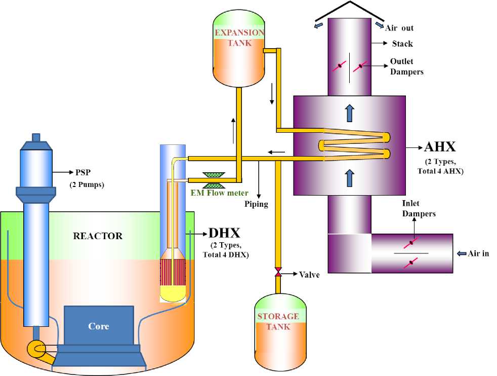
Fig. 1: Simplified Schematic of SGDHR System of PFBR

The SGDHR system comprises of many components; with redundancy in design for increased reliability. It is a passive standby system for decay heat removal which is called into operation when the normal active heat removal path, through Operational Grade Decay Heat

Removal (OGDHR) system is unavailable. For successful decay heat removal both Primary Heat Transport and SGDHR should work. So, the components in primary sodium circuit (like pump, motors), intermediate sodium circuit (Direct Heat

For PFBR Test Interval data has been given from experience of previous fast reactors, this value can be improved with further cost reduction without affecting the unavailability. The cost values are only representative in this study. The reliability analysis was done [3] and fault trees [4] for Primary Circuit, Intermediate and air circuit were considered.

• III.    Equation Formulation

Models for unavailability and cost of testing of individual components are established with Surveillance Test Interval as decision variable. Reliability parameters like standby failure rate, per demand failure probability, mean time to test, testing cost per hour, mean time to repair and cost of repair per hour are considered for modeling. The list of symbols used to represent reliability parameters testing and maintenance of whole system is found by adding individual component costs and the system unavailability is found by adding the minimal cutsets derived from the fault tree analysis of the system. These models for system cost and unavailability serve as objective functions that have to be minimized by deciding on the values of test and maintenance intervals.

Table 1: Reliability Related Symbols Used

Symbol	Meaning
T	Surveillance test interval
t	Mean time to test
λ	Standby failure rate
T R	Mean time to repair
C ht	Surveillance Testing cost per hour
C hr	Cost of repair per hour

The unavailability equation for a periodically tested component of SGDHR system was formulated as:

«ito = Л (JJ2 + Г_я)

where ui(x) represents unavailability of ith component(or basic event) that depends on the vector of decision variables x and Ti represents the test interval for ith component(or basic event). In this study, we are optimizing based on the value of test interval, so x has a single decision variable that is Ti. Total system unavailability was found from the cut-set equations obtained from the fault tree analysis, and is given as the sum of j number of minimal cut sets, each with the product k extending to the number of basic events in the jth cut set:

Uto =1)П_ки^ (2)

where U(x) is the total system unavailability that depends on test interval values of all the components in the system and ujk represents the unavailability associated with the basic event k belonging to minimal cut set number j. The cost model is established as:

Cito = —С^* АТ_Н С_гл (3)

The total yearly cost of the system having i number of components is given by:

Cto = Ei с, (x)

The problem is solved using GA for two cases:

Case 1: Keeping the cost as objective function to be minimized and unavailability as constraint. That is represented as:

^(E^i Cj (x))

(7(x)

Case 2: Keeping the unavailability as objective function to be minimized and cost as constraint. That is represented as:

Min(U^

Ep₌₁c_i(x) < MaxCost

For the high redundancy systems like SGDHR, data for large number of simultaneous failures does not exist. So, a common cause analysis is done with beta factor model, in which common cause failure (CCF) rate is obtained as a fraction (Beta) of single component failure rate. The value of beta is assumed to depend on the number of such redundant components. The approach followed in this study is that active components with levels of redundancy less than or equal to three, a beta of 5% is used. If redundancy is greater than or equal to four, a beta of 1% is used.

• IV.    Genetic Algorithm Design - Overview

In a genetic algorithm, many individual solutions are randomly generated to form an initial population. This population then evolves over successive generations to give better solutions. Each generation comprises of various phases, the most important being – fitness evaluation, selection (competition), reproduction (crossover) and mutation [5]. Fig. 2 shows the control flow of GA for a constrained problem with fitness penalization. Initial population is generated which is a collection of many solution vectors or individuals. Each solution vector comprises of the test intervals of all components being tested which are represented by T1, T2, T3…Tn. These are the decision variables whose value is to be decided by GA such that the objective functions’ value reaches optima. In the fitness evaluation step, quality of each individual is assessed based on the objective function. Then each individual is checked for constraint violation where a constraint may be implicit i.e. the value of the individual lies outside the defined range or it may be explicit i.e. it requires evaluation of a function. If an individual violates the constraint then its fitness is reduced in the penalization step. Then the termination criteria are checked. Selection, crossover and mutation operators are applied to the population as discussed in section V. This process is repeated until the maximum number of generations is reached which is the termination criterion for our study.

An individual is represented as a string of numbers known as a chromosome. Chromosomes are composed of genes where each gene is a set of values called alleles that represents an encoded decision variable. Real value representation is used here for test interval optimization; as it has the property that two points close to each other in the representation space must also be close in the problem space and vice versa. It is also conceptually closest to the problem space and allows easy and efficient implementation of closed and dynamic operators. Test Interval (TI) values are given in hours and the maximum bound on each component’s Test Interval value is 8760 hours, which corresponds to 1 year.

Goldberg DE [6] suggested that good GA performance requires the choice of high cross over probability, low mutation probability and a moderate population size. For all the experiments, crossover rate of 0.6 was taken. Mutation rate of 0.002 was found to be the best for cost optimization and a rate of 0.03 was found suitable for risk minimization, based on a number of trials. Population size was taken as 100 for each case and GA was run for 10000 generations.

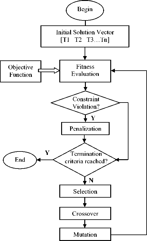
Fig. 2: Control Flow of GA

• 5.1    Fitness Evaluation

• 5.2    Penalization

GA is implemented for TI optimization with the following methods and operators:

Fitness evaluation is the step in which the quality of an individual is assessed. An individual is decoded and its cost and unavailability are found using the models in (2) and (4), as described in section III. Fitness is evaluated as the inverse of cost or unavailability depending on which one is taken as the objective function. In this way, the problem is converted into a maximizing one by taking the fitness function as the reciprocal of the actual function value that is to be minimized.

Optimization of test schedules is done by taking either cost or unavailability as the objective function and the other as the constraint. Penalization is the process of converting a constrained problem into unconstrained one by reducing the fitness of solutions that violate the constraint. Here, we have implemented a dynamic penalty function, as suggested by Martorell [2], where the penalty value depends on the amount of constraint violation and generation number of GA. This penalty function is given as:

where the parameters α and β are defined by the user and K(g,α) is an α-function that establishes the pressure on infeasible individuals taking into account the number of generations evolved, g. SVC( β, i) is a β-function that represents the sum of violated constraints for a given individual i, which is formulated as follows:

SVC (8,0 =^D.^S(i} (10)

The sum in (10) extends to the total number of constraints to which each individual, i, is subjected, where for a given constraint, j, the corresponding D* (0 is defined by the expression:

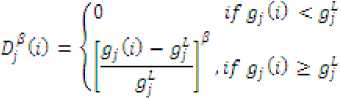
which represents the degree of violation associated with restriction j, where gj(i) represents the value achieved by the individual i with regard to constraint j, whereas Sj is the maximum value allowed for this constraint j.

The dynamic penalization feature is provided in this solution using an appropriate function K (g, α). The pressure on infeasible individuals has to rise as the number of evolved generations increases. Different expressions for K (g, α) have been proposed. In this solution, the function selected is given by:

K(g.cO = ^[(5 - l).p + l]^c (12)

where g corresponds to the current generation number, and K1 and p are the two parameters to be determined according to the desired values of δ1 and δGs , and the number of generations, Gs, for a given μs, as:

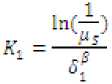
Suitable values for δ1, δGs, Gs and μs are 0.01, 0.001, 1000 and 0.01, respectively. In addition, common values for the couple (α, β) include (0.5, 2), (1, 2) and (2, 2).

In our GA, the function used to penalize infeasible solutions is a variation of the family functions described by (9). This function introduces penalization relative to the worst score encountered in the population after the evaluation stage for the current generation, which also depends on the number of generations evolved, g. Thus, the penalized objective function for a given individual, i, is as follows:

f' G) = f(0 ± [1 - u(a, /?, 0 ]./(w) (15)

where f(i) represents the raw score of the initial objective function for the individual i, and f(w) is the corresponding score for the worst individual found in the population at current generation g. The sign of (15) differs whether the objective function is minimized or maximized. In the former case, the penalization is added to the initial objective function score, while it is subtracted otherwise.

• 5.3    Fitness Scaling

• 5.4    Elitism

• 5.5    Selection

• 5.6    Mutation

Linear Fitness Scaling was introduced to improve the performance of GA by controlling copies of individuals in the beginning of run and as the run matures, thereby preventing convergence to suboptimal solutions. If the raw fitness is defined as f and the scaled fitness as f’ then linear scaling is a linear relationship between f’ and f as follows:

f = a* f-b (16)

The coefficients a and b may be chosen in a number of ways; however in all cases we want the average scaled fitness f’avg to be equal to the average raw fitness favg because subsequent use of the selection procedure will ensure that each average population member contributes one expected offspring to the next generation. To control the number of offspring given to the population member with maximum raw fitness, we choose the other scaling relationship to obtain a scaled maximum fitness, f’max = Cmult.favg, where Cmult is the number of copies desired for the best population member. For typical small population (n = 50 to 100) a Cmult = 1.2 to 2 has been used successfully.

Toward the end of the run, this choice of Cmult stretches the raw fitness significantly. This may in turn cause difficulty in applying the linear scaling rule. At first there is no problem applying the linear scaling rule, because the few extraordinary individuals get scaled down and the lowly members of the population get scaled up.

This was implemented to retain the best individual of a generation in the next generation so that highest fitness solutions are not lost in reproduction and mutation. For this a single individual with highest fitness from the current generation’s population is copied directly to the population in the next generation.

Selection is an operation used to decide which individuals to use for reproduction and mutation in order to produce new search points. For the purpose of this study we have implemented Roulette wheel selection scheme that samples the individuals by simulating the roulette-wheel for fitness proportionate selection.

Mutation is normally applied to one individual in order to produce a new version of it where some of the original genetic material has been randomly changed. By itself, mutation is a random walk through the string space. When used sparingly with reproduction and crossover, it is an insurance policy against premature loss of important information. Here, we have implemented non-uniform mutation which is a dynamic mutation operator aimed at both improving singleelement tuning and reducing the disadvantage of random mutation in the real representation. For a parent TIgen, where TI is Test Interval and gen is generation number, if the kth element TIk,gen was selected for mutation, the resulting offspring is:

• Tb - TZ ■ )

• V          if a random digit is 1

• 5.7 Crossover

• 5.7.1    Arithmetical Crossover:

• 5.7.2    Blend Crossover (BLX-a):

The delta function above is denoted in a general form as - Δ (t, y), which returns a value in the range [0, y] such that the probability of Δ (t, y) being close to 0 increases as t increases (here we have used t as the generation number). This property causes the operator to search the space uniformly when generation number is small and then very locally in the later stages. The following functional form has been used:

where r is a random no in the range [0, 1], T is the maximal generation number, and b is a system parameter determining the degree of non-uniformity. Non-uniform mutation causes global search of the search space at the beginning of the iterative process, but an increasingly local exploitation later on. This is suited for a problem where the number of feasible solutions in the space is very small.

Reproduction is the process by which the genetic material in two or more parent individuals is combined to obtain one or more offspring. For the purpose of comparison the following crossover schemes were considered:

This operator is used in real representation and is defined as a linear combination of two vectors (chromosomes) [7]. If the parent solutions       and are to be crossed, the resulting offspring are:

where ‘a’ is random no. in the range [0, 1], as it always guarantees closure (                        ).

Such a crossover is called average crossover when a = ½. The average value of the selected parents is calculated (with a=0.5) and assigned to the offspring chromosomes as follows:

This is also known as BLX-α crossover [8] and has been used with real representation. For two parent solutions        and       , if         and         are genes to be crossed (assuming       <      ), then

BLX-α randomly picks a solution in the range "^Kgen ^— ®(T^kg«T. ^— TI^gg^yTl^gir + О(ТЬ_Лд,_Г -T1. Л

Thus, if u is random number between 0 and 1, following is the resulting gene in an offspring:

where                      . BLX- α has an interesting property that the location of the offspring depends on the difference in parent solutions. This will be clear from the equation below:

Test Interval Optimization for Nuclear Power Plants

If the differences between the parent solutions are small, the difference between the offspring and parent solution is also small. This property of the search operator allows us to constitute an adaptive search. Thus such an operator allows us the searching of entire space early on (when a random population over entire space is initialized) and concentrate the search more on the later stages when the population tends to converge in some region of the search space.

• VI.    Selection Of Suitable Crossover Mechanism

• 6.1    Choosing a Value for Blend Crossover:

• 6.2    Comparison of Arithmetical and Blend Crossover:

For this study, the crossover for Real-parameter Genetic Algorithm was implemented in two different ways –Arithmetical crossover and BLX-α crossover – to make a comparison of their performance. The value of alpha parameter of BLX-α was first selected based on a number of trial runs for cost minimization with Common Cause Failure (CCF) and without CCF. Then with this value fixed in BLX-α, a comparison was done for arithmetical and BLX-α crossover. For cost minimization, the results are given as the minimum cost of testing per year in Indian Rupees; for unavailability minimization, the results are given as the minimum unavailability per demand.

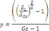
Cost optimization was done using GA for different α values (α = 0.1, 0.2…0.9) of BLX-α crossover, each with the same initial population (generated by using the same seed for random number generation) keeping the other GA parameters fixed. This was repeated for ten different sets of initial population i.e. ten different trial runs and the results for each α value were averaged and plotted as shown in Fig. 3 and Fig. 4 for components with CCF and without CCF, respectively. It is clear from these figures that BLX-α performed better with α value of 0.4 for cost minimization with CCF and value of 0.5 for cost minimization without CCF. Hence, we selected these values for further analysis.

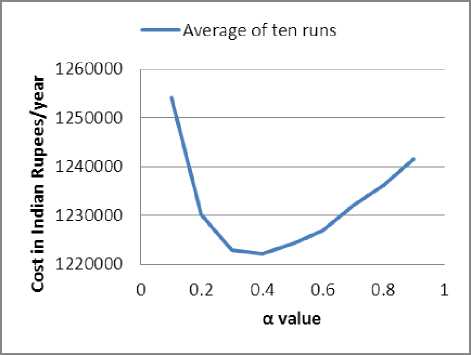
Fig. 3: BLX-α crossover with CCF

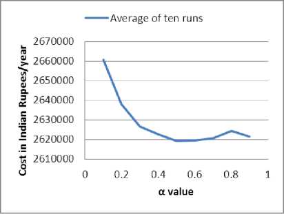
Fig. 4: BLX-α crossover without CCF

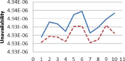
The arithmetical and BLX-α crossover were employed for optimization, each with the same initial population, over ten trials (i.e. ten different sets of initial population). Here, BLX-α crossover’s alpha parameter was set to 0.4 for cost minimization with CCF and to 0.5 for all the other cases. The results obtained were plotted in Fig. 5, Fig. 6, Fig. 7 and Fig. 8 for cost minimization with CCF, cost minimization without CCF, unavailability minimization with CCF and unavailability minimization without CCF, respectively. It can be noted that the curve for BLX-α lies below the arithmetical crossover for all the cases, showing a better performance.

Fig. 5: Cost minimization with CCF

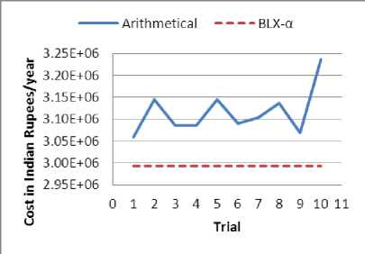
Fig. 6: Cost minimization without CCF

Test Interval Optimization for Nuclear Power Plants

------Arithmetical ----BLX-a

Trial

Fig. 7: Unavailability minimization with CCF

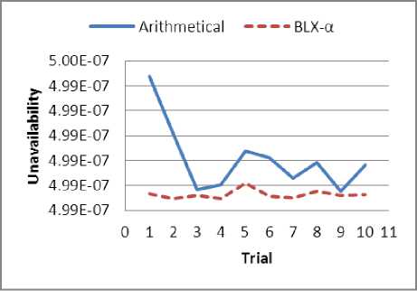
Fig. 8: Unavailability minimization without CCF

• VII.    Results and Discussions

The results for cost minimization with CCF and without CCF are significantly better for BLX-α compared to arithmetical crossover as shown in Table 2. For unavailability minimization the difference between the results obtained with BLX-α crossover and arithmetical crossover is small, but BLX-α crossover produces better results than arithmetical for the same initial population. In general the better performance of BLX-α is due to its implementation that allows for generating offspring in the neighborhood outside the two parent solutions as well, rather than taking only the interpolated values between two points. This is helpful when the problem is multimodal i.e. there exist more than one solution to the problem. Whereas, arithmetical crossover is more suitable for problems that have a single mode and which can be represented by constantly increasing or decreasing functions. Also, BLX-α allows for better exploration of the search space and is suitable for problems that involves non-linear objective functions and/or constraints, like ours.

Table 2: Optimized Results with Different Crossover Mechanisms

S. No.	Case	Optimum value obtained from
		Arithmetical Crossover	BLX-α crossover
1	Cost Min with CCF	1432570	1395360
2	Cost Min Without CCF	3059780	2993220
3	Unav Min with CCF	4.93157E-06	4.93023E-06
4	Unav Min without CCF	4.98975E-07	4.98947E-07

• VIII.    Conclusion

Here, we considered the problem of deciding test intervals for a safety critical system of PFBR, wherein the test strategy for the plant was improved such that unnecessary testing burdens are reduced without compromising the plant safety. The reliability parameters values were taken from an internal report [3] and serve as input data for solving the unavailability and cost equations, (2) and (4). Two separate optimization cases were considered namely cost minimization and availability maximization. The optimization was done using Genetic Algorithms which takes cost or availability as the objective function and solves for the set of best test interval values for all components. We have done a comparative study on two different crossover implementations namely arithmetical crossover and BLX-α crossover. Firstly, the ‘α’ parameter of BLX-α was fixed by comparing the optimum results obtained with different α values. It was found that α = 0.4 gave better results for cost minimization with CCF and for all the other cases α = 0.5 was found more suitable. The suitable values of α were used with BLX-α crossover and the different crossover mechanisms were evaluated for each case. BLX-α crossover was found to perform better than arithmetical crossover for this problem domain.