Sugarcane crop yield forecasting model using supervised machine learning

Published Online August 2019 in MECS

Long Term Time Series (LTTS) forecasting has been a useful tool for governments, planning commissions and decision makers in various applications such as solar energy, wind power energy, economic forecasting, and in the agriculture sector. Historically, LTTS has been applied at the regional and national level for planning, import and export decision making and policy decisions[1,2]. Traditionally, application of LTTS in the agriculture sector for yield prediction/crop forecasting is limited to empirical methods using ground-based observations and productions reports gathered by various organizations from different sources: meteorological data, agro-meteorological(yield), soil (water holding capacity), and remotely sensed agricultural statistics. Based on meteorological and agronomic data, several indices are derived which are deemed to be relevant variables in determining crop yield. For instance, crop water satisfaction, surplus and excess moisture, average soil moisture. As Crop production rate depends on the geography of a region(e.g. hill area, river ground, depth region, etc), weather condition (e.g. temperature, cloud, rainfall, humidity etc), soil type (e.g. sandy, salty, clay, peaty, saline soil etc), soil composition (e.g. PH value, nitrogen, phosphate, potassium, organic carbon, calcium, magnesium, sulphur, manganese, copper, iron etc) and harvesting methods, various combinations of subsets of these influencing parameters have been used by different prediction models for crop yield prediction using groundbased observations[3-7]. Prediction models are broadly classified into two types: i)traditional statistics model (e.g. multiple linear regression model), which formulates a single predictive function holding entire sample space. i.e. it generates a global model over the entire sample space. ii)machine learning technique, which is emerging technology for knowledge mining that relates input and output variables which is hard to obtain statistically. In traditional statistical methods, the structure of the data model needs to be assumed priory, whereas machine learning techniques need not assume this structure. This is a useful characteristic for machine learning techniques to model complex, non-linear behavior in crop yield prediction. Recent researches in the field of yield prediction have focused on Remote Sensing(RS) data and Machine Learning(ML) techniques, as RS data is cost effective compared to ground observation data. RS data, such as Special Vegetation Indices (SVIs) derived using multi hyper-spectral calibrated data. The one among is the Normalized Difference Vegetation Index(NDVI), a type of SVIs, used with machine learning parametric algorithms like Linear Regressions, Naïve Bayes,

Gaussian Process and Simple Neural Networks, as well as non-parametric algorithms like Support Vector Machine(SVM), Decision Trees(DT) and Nearest Neighbors to predict yield successfully. Parametric ML algorithms are derived from traditional statistical methods. The latest development in yield prediction being an application of Deep Learning(DL) techniques using RS dataset[8,9]. NDVI is calculated as normalization of reflectance values from Near Infrared(NIR) and red brands ranging from -1.0 to +1.0. Higher NDVI is an indication of greener surface and lower NDVI indicates less green surface[10]. Crop yield has been predicted not only at the beginning of the sowing phase but also at various intervals and phases during crop cultivation season depending on purpose and organizations. ^

As defined by the Food and Agriculture of the United Nations, crop forecasting is the art of predicting crop yields and production before the harvest actually takes place, typically a couple of months in advance[11]. Defining time horizon for crop yield forecasting in terms of time series forecasting methodologies is an important aspect. In common research practice, forecasting horizons are categorized as short-term, medium-term and longterm. Short-term forecasting horizons are closer to the end of observation time period, and long-term forecasting horizons are far from the end observation time period [12, 13]. In other words, single step forecasting is short-term, two steps forecasting is a medium-term and more than two steps forecasting is long-term forecasting, where a step is time unit of observations, like a month in monthly observed time series. In many applications of time series, the boundary for categorization of time series forecasting may not be defined clearly. Total yield being a one-time outcome in season, time horizons for yield prediction needs to be defined with different parameters to be predicted for meaningful results. Yield prediction could be useful in achieving maximum yield rate of the crop using the limited land resource as part of agricultural planning in an agro-based country [10]. Antecedent determination of problems associated with crop yield indicators can help to increase the yield rate of crops. Crop selector could be applicable to minimizing losses when unfavorable conditions may occur and this selector could be used to maximize crop yield rate when the potential exists for favorable growing conditions. Maximizing production rate of the crop is an interesting research field to agro-meteorologists which play a significant role in the national economy[14]. In India, farmers' conditions are worsening day by day, even during favorable condition as well as unfavorable condition. During favorable condition, with bumper yield, farmers are getting less price because of surplus yield than demand. During unfavorable condition, because of loss of crop. Crop yield prediction could be useful in selecting crop to minimize loss to farmers'.

Forecasting Agricultural output using Space, Agro-metrological and Land based observations (FASAL)[15], forecasts multiple in-season yields, namely pre-season, early-season and mid-season. Recent developments in FASAL shows that it is able to predict statewide yield using Lasso Regression with an accuracy of about 80%[15]. FASAL combines conventional methods of forecasting with remotely sensed data to make multiple in-season yield predictions. Applications of predictive empirical models using remotely sensed data in crop yield prediction have been popular, and successful in predicting yield efficiently and quantitatively. Previous studies have established that NDVI data which is derived from satellite images, normally used for monitoring vegetation health and changes in growth patterns, could be used for in-season yield prediction in a larger region. Many researchers have also established a relation between various weather parameters, such as surface temperature, precipitation, soil moisture and cloud cover with NDVI values. Past research studies in soil parameters, weather, NDVI and yield predictions have shown a strong relationship between these four types of parameters. Although previous studies have successfully applied various machine learning algorithms to crop yield prediction considering NDVI, weather parameters and soil parameters as attributes, inherent dependencies of these attributes requires careful selection of these attributes to address curse of dimension problem in machine learning.

• II.    Related Works

Crop yield forecasting is a unified, bio-socio-system comprised of a complex interaction among soil, air, water, and crops grown in it, where a comprehensive model is required. Crop yield forecasting models could be categorized based on attribute measurement methods, such as ground-based observed data, remotely sensed data, and a combination of both ground-based and remote sensed. Another way to categorize yield forecasting models could be as classical empirical models and machine learning models[1-7]. Researchers have been using periodical, cost-effective and comprehensive remote sensed data, which provides information about earth surface for yield prediction. Two approaches have been used to obtain a quantitative relationship between remotely sensed data and crop yield. Studies in the first group of approaches incorporate remotely sensed data into agro-meteorological models such as SAFY and Aqua Crop [16]. These approaches predict yield accurately and model crop development, but requires large amount and complicated field inputs like water balance models, fertilizers, etc. derived from remotely sensed data. The second group of classical approaches to yield forecasting is based on empirical relationships like regression. Advanced ML techniques[17], Adaptive Neuro Fuzzy-Inference Systems [18], Multi-Layer Perceptron (MLP), Artificial Neural Network (ANN) [19], Bayes Net, XY-Fused Networks, Supervised Kohonen Network, Counter Propagation ANN, have been applied in yield prediction for yields like rice, wheat using various indices like NDVI, SVI and LAI [20, 21].

India is the second largest sugarcane production country in the world. Sugarcane is cultivated across all states in India and across different seasons. India has most of its sugarcane cultivation located on the subtropical belt, Uttaranchal, Bihar, Uttar Pradesh, Punjab, and Haryana are important sugarcane growing states in the Indian sub-tropical region. Sugarcane is also grown in a few minor regions and pockets of Madhya Pradesh, Rajasthan, Assam, and West Bengal, but these states have a low throughput when compared to the sub-tropical and tropical belts. The growth of sugarcane is massive and expansive in the tropical belt and states such as Maharashtra, Tamil Nadu, Andhra Pradesh, Karnataka, and Gujarat, as sugarcane is a tropical crop, thus all the agro-climatic conditions for the cultivation of sugarcane are met at these states. Growth Cycle of sugarcane yield plays a very important role in crop yield prediction. So, in this section, we discuss the conditions favorable for sugarcane growth along with the crop cycle. Depending upon the sowing time and variety of the crop, it takes about 12 to 18 months for sugarcane crop to mature. Generally, the months of January to March are considered for sowing, and harvesting is done from December to March. Once harvesting is completed, a ratoon crop is cultivated from the re-growth. A Ratoon Crop is the new crop which is cultivated using the stubble left behind from the previous harvest. In India, it is a common practice to take one ratoon after a normally planted crop. In a few countries, 2-6 ratoon crops are allowed[22]. Sugarcane demands high water and high nutrient consumption for a long duration. The range of climatic conditions where sugarcane will be grown is wide, sugarcane is grown ranging from sub-tropical to tropical conditions. Temperatures below 20oC and above 50oC are not suitable for sugarcane growth. For optimum productivity, the requirement of 750-1200mm of rainfall needs to be satisfied during the growth period. Well-drained alluvial to medium black cotton soils with neutral pH (6.0-7.0) and optimum depth (>60 cm) are good for sugarcane growth. Optimum productivity is also being obtained in sandy to sandy-loam soils with near neutral pH under assured irrigated conditions of North India[22-27]. Sugarcane planting could be done in three seasons namely, Spring, Winter, and Adsali. Spring planting is also called as "Suru", is done during January to February, Winter planting, also called as "Pre-Seasonal" planting, is done during October to November, and Adsali planting is done during July to August[22].

In this paper, we are proposing novel crop yield forecasting model using long term time series and support vector regression, for sugarcane as a primary crop in a multi-crop system with multiple, unknown inter-season secondary crops, using remote sensed NDVI data and ground-based observed, highly co-related weather and soil data. We are also comparing the accuracy metrics of SVR with other popular supervised ML algorithms like Gaussian Process Regression(GPR)[23] and Linear Regression(LR). Parametric ML algorithms, GPR and LR have been chosen for comparison purpose because of their derivation from classic empirical models. We are also analyzing curse of dimension problem of ML algorithms by using dimension reduction techniques like Lasso Regression ML algorithm[24] as well as selecting the various combination of attributes using correlation matrix and feature selection techniques.

This paper is arranged as follows. Section III describes sugarcane crop cultivation in India, Section IV outlines dataset used for yield prediction and dataset preprocessing. In section V, modeling time series dataset as a supervised ML problem and implementation of long term time series yield prediction model are explained, in section VI, we have discussed experimental results and analyzed the impact of the curse of dimensionality on sugarcane yield prediction outcome using SVR and other popular supervised ML algorithms, and section VII concludes this paper and lists the scope for future enhancements.

• III.    Sugarcane Crop Cultivation in India^

Fig.1 shows the Gantt chart for sugar cultivation in India.

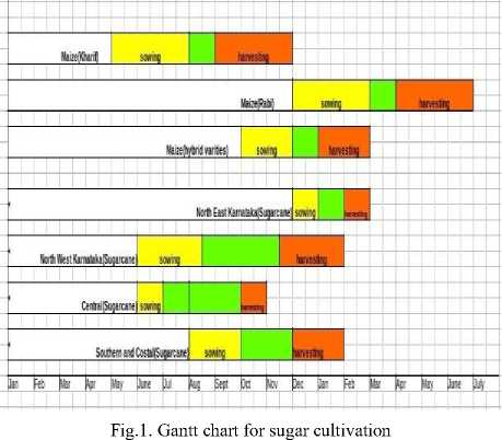
As sugarcane is cultivated by planting in either January-February, July-August or October-November, with maturity duration of 12-18 months, it is challenging task for predicting crop yield, as time series problem across various states of India. In Karnataka and Maharashtra states, sugarcane variety with 12 months maturity is cultivated, whereas for different sub-regions planting time varies. SCLC has four phases, a)Germination and Establishment, b)Tillering, c)Grand Growth, d)Ripening and Maturity. Germination and Establishment phase lasts for 15 days, whereas Tillering phase is for about 4 months, Grand Growth phase is about 4.5 months, Ripening and Maturity phase lasts for 3 months. As plantation start time varies in the Karnataka region, start and end of each phase vary in different regions[22].

• IV.    Dataset Description

Dataset is a critical component of any ML algorithm and it needs to be understood and pre-processed before applying ML algorithms in any domain. Dataset used in this research comprises Weather and Soil Dataset(WSD), NDVI dataset and Sugarcane crop yield dataset. WSD is downloaded from .246N74.737E [28], for the village Shirdhan, located at latitude and longitude of 16.2458oN, 74.737oE of Belagavi district, Karnataka(India). WSD dataset attributes are listed in Table 1.

Table 1. List of attributes and units of measurement

Attribute Name	Measurement Units
Temperature (2m above ground) (T)		Celsius
Dew Point Temperature (2m above ground) (DPT)		Celsius
Soil Temperature (0-10cm below ground) (ST)		Celsius
Soil Moisture (0-10cm below ground) (SM)		m 3. m- 3
Precipitation (P)		mm
Relative Humidity (2m above ground) (RH)		%
Sunshine Duration (SD)		W/ m 2
Evapotranspiration (E)		mm
NDVI		range(-1 ,1)

pn FebMarApr Maj-fun Jj Aug Sep to tor Dec Jan Feb Mar Apr May jin pl Aq Sep to tor Det Jan Feb Mar Ayr May Jr, pl Aq Sep Oct tor Det

pn Feb «v Apr way ^n jj AiqSeptotorto Jm Feb *tor Apr Kty Jun pl AqSepOcttorDec Jan Feb*r Vtoyjxi pl Aug Sep to tor Dec

pfifebH3f«pftoyjwi J^ AjqSeptotoyto jr Feb Mw Apr №fy jw pl *q Sep Oct tor Dec jv Feb ««toy Jr pl №g Sep Oct tor Det Month                                              Month                                              Mofffi

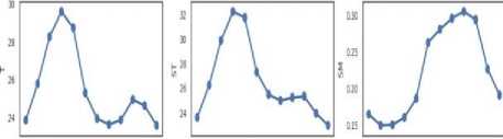
Fig.2. Yearly Average Weather and Soil Attributes at Location Shridhan with nine subplots for each attribute. T-Temperature, ST-Soil Temperature, SM-Soil Moisture, SD- Sunshine Duration, EEvapotranspiration, P-Precipitation, RH- Relative Humidity, DT-Dew Temperature, NDVI - Normalized Difference Vegetation Index.

WSD dataset consists of ground-based observed data hourly for the last 30 years. Remote sensed NDVI values are derived from LAND SAT II images captured for every 15 days between the years 2008 to 2018, and total yield-per-hector, number of hectors cultivated for entire Belagavi district are gathered from the website [29] and adjusted the values based on a ground survey at a different location. We have dataset with NDVI values observed at every 15 days for 8km x 8km region, weather and soil data recorded at every hour at latitude and longitude, and yield per hector with number of hectors cultivated, gathered at every season of primary crop sugarcane and secondary crops like maize, rice for entire district, where season for sugarcane is entire year and for secondary crops, three seasons in a year.

Fig.2 shows the average yearly pattern of each attributes at Shirdhan. Temperature and Soil Temperature follows a similar pattern. Soil Moisture, Relative Humidity, and Dew Temperature follow similar trends, Sunshine Duration and Precipitation follows the opposite trend. Closely looking at NDVI trend, which is lowest during January and highest during September and October, and starts reducing during November and December. So we can safely assume that crop sowing starts during January and harvesting starts during November.

• A.    Dataset Distribution And Outliers

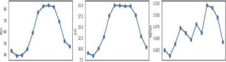
Using various graphs, we can understand the distribution of each attributes in dataset independently. Box and Whisker plot is shown in Fig.3, indicates weather attributes are skewed or have outliers. Attributes like Precipitation, NDVI, and Evapotranspiration have outliers. Outliers in weather dataset could not be neglected, as they provide very important information about the nature of overall weather condition. Histogram graph, as shown in Fig.4, groups each attributes in the number of bins and provides the number of observations in each bin, and shape of bins lets us understand the kind distribution each attribute is following.

Fig.3. Box and Whisker Plot^

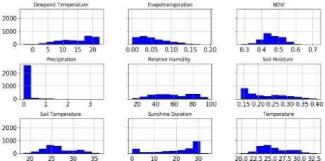
Fig.4. Histogram graph.

• B.    Correlation of Attributes

Correlation Matrix as shown in Fig.5 establishes a relation between various features. ML requires features to be independent for better learning. From Fig.5, it is clear that attribute Temperature has a positive relationship with Soil Temperature and Dew Point Temperature, negative relation with Soil Moisture, Relative Humidity, Evapotranspiration, and Precipitation. After careful analyses of the correlation matrix, we could select either Temperature or Soil Temperature, either Dew Point Temperature or Relative Humidity, either Sunshine Duration or Soil Moisture. Correlation matrix also conveys that, many features have a strong relationship between them. So feature selection or dimensionality reduction should be applied before learning prediction function. Criteria for Selection of attributes in high dimensional dataset, feature selection or dimension reduction techniques have been used to reduce feature to boost algorithm performance, increase the accuracy of estimators. Univariate feature selection method selects the best feature based on statistical tests like best scoring feature, best percentile feature, false positive rate, false discovery rate, family-wise error, hyper-parameter search estimator. Recursive feature elimination method, which eliminates features by comparing a small set of features recursively, L1 based feature selection methods based on linear regression and Linear SVM, Tree-Based Feature Selection compute feature importance. In this paper, ML-based feature selection methods are used to calculate the importance of each feature.

Fig.5. Correlation matrix.

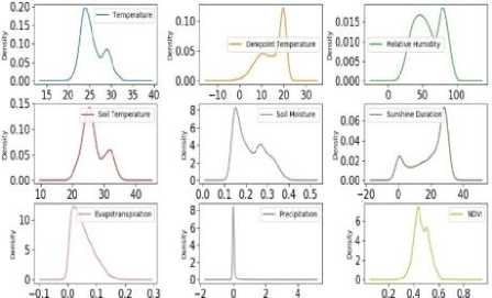
Fig.6. Density graph.

• V.    Sugarcane Yield Prediction Model

Proposed Sugarcane Crop Yield Forecasting Model(SCYFM) consists of three modules, which are in accordance with ML approaches. As shown in Fig.7, the first module known as Dataset Pre-processing Module(DPM) re-samples, scales and normalizes each attribute, select independent and important attributes and divides into training and testing dataset. The second module i.e. Training and Testing Module(TTM) trains SVR algorithm with RBF kernel and other Supervised ML algorithms for comparison purpose, and verifies trained algorithms using hold-out data and compares various regression metrics to evaluate efficiency and accuracy of a trained module. The third module is known as Prediction Module(PRM) forecasts weather and soil attributes, NDVI, and finally sugarcane crop yield. Each module has three sub-modules: Weather and Soil Attribute Module(WASAM), which deals with weather and soil attributes pre-processing, training, testing, and prediction. NDVI Module(NDVIM) for NDVI values, and Sugarcane Crop Yield Forecasting Module (SCYFM) for sugar- cane yield. All three modules are implemented using Sci-Kit Learn package version 0.1.91 and Python 3.7.

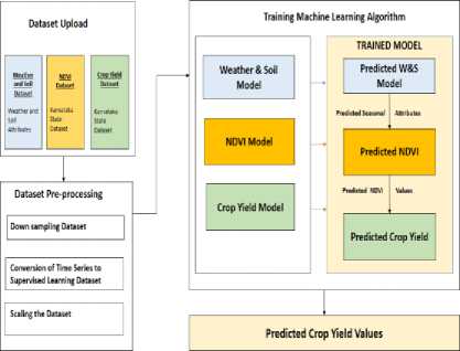
Fig.7. Architecture Diagram of the proposed model

• A.    Dataset Pre-processing Module

Forecasting weather and soil attributes for the duration of 12 months SCLC, hourly observation is not a practically feasible solution as it would require to model long term series of 24 x 365 steps supervised ML problem, hence weather and soil dataset needs to be resampled to NDVI observation. Re-sampling methods such as Down-sampling, where the frequency of observation is decreased from hourly to daily, and/or Upsampling, where the frequency of observation is increased from monthly to daily, could be used to bring observations to the same frequency. In up-sampling, minute observations are calculated using interpolation, whereas in the case of down-sampling, aggregated observations are calculated using summary statistics. In WASAM sub-module of DPM, weather and soil dataset have been down-sampled from hourly to 15 days aggregate, which is the frequency of NDVI values. After down-sampling, weather-and-soil time series dataset is converted to 24 steps supervised ML dataset and every 15-days observation is considered as one feature. The dataset for supervised learning consists of input and output attributes, and ML algorithm learns function which relates output(s) to input attributes. Time series dataset consists of observations indexed by time period, i.e. frequency, but observation at frequency 't' is independent and identically distributed. However, observation at frequency 't' depends on observation at previous frequency t-1 in the long term and has a regular pattern. So observation at time 't+1' will be dependent on observation at a time 't', by considering this, we have converted time series dataset into supervised machine learning problem.

NDVI Forecasting for the duration of SCLC, 12 months is considered as supervised ML problem with NDVI values as output and WS attributes as input. WS dataset has been down-sampled to the frequency of NDVI, but each attribute is measured on a different scale. In NDVIM submodule, attributes are scaled between 0 and 1 using normalization according to equation (1)

NXi =

xi  x min

X — X- max   min

NXi is the normalized value of observation Xi, xi is the value of ith observation for attribute x, xmax is the maximum value observed for attribute x and xmin is the minimum value observed for attribute x. SCYFM is considered as a ML problem with sugarcane crop yield as output and NDVI values as input. Crop yield is recorded at every season, where the season is 12 months long and NDVI values are derived after every 15 days. We have four years of yield data per district, which makes it difficult for the ML algorithm with one district dataset. So we have considered all sugarcane growing districts in Karnataka state for training and testing purpose, whereas yield is predicted at Shirdhan. Mean, Median, and Standard Deviation of NDVI values for each phase of sugarcane cultivation is considered as one input attribute. Phase wise NDVI aggregation is done according to planting timing in each district. In Bijapur and Belagavi districts, sugarcane planting is done in January, So NDVI for first 15 days of January is considered as phase 1 NDVI, whereas in Coastal districts, planting is done in November, so NDVI for first 15 days of November is considered as Phase 1 NDVI. Phase 2 NDVI values are calculated as aggregate of NDVI values of the next four months after the first 15 days of January and November respectively for each region. Phase duration for different regions in Karnataka is shown in Fig.1.

• B.    Training And Testing Module

In WASAM submodule, each attribute listed in Table.1 is observed at every hour, down-sampled to every 15 days, and are forecasted individually for the duration of one year by modeling 24 steps LTTS as supervised ML regression. WASAM is trained iteratively as SVR algorithm with RBF kernel, C value as 100 and gamma value as 0.1, using previous 20 years observations over a prior 6, 12, 18, and 24 observations as input set and next 24 observations as multiple outputs. Learned Model has been tested using held-out dataset samples of 75% to 5% of total samples. In NDVI module, weighted SVR algorithm is trained using previous 8 years of WS and NDVI datasets, where WS dataset is recorded every hour and down-scaled to every 15 days, as input attributes and NDVI dataset is observed every 15 days as output to forecast NDVI as a time-independent attribute. In practice, NDVI is derived from greenery and solar radiance and is not time-dependent as weather and soil. Weights of samples are increased in accordance with the chronological order of dataset, with an assumption of recent past WS attribute values have more influence as compared to past values. According to the correlation matrix, it is observed that WS attributes are completely independent, and in order to reduce the influence of dependent attributes, feature selection algorithms like Lasso, Decision Trees are used to select the best features. NDVI module has been trained and tested with various combinations of features. In CYPM module, SVR algorithm is trained using average NDVI values for the past 8 years from 28 districts of Karnataka state, where sugarcane is cultivated, as a dataset with NDVI at every 15 days over one year period as input attributes and yearly sugarcane crop yield as output. If we consider one location then dataset will have only 8 samples, so all districts of Karnataka is considered for training SVR. In this module, training dataset has been divided into various sizes between 20% and 90% in the step of 5% each, and comparison of training time and r2 score values have been analyzed to understand the minimum number of training samples required for better accuracy. Other ML algorithms like GPR, DT, and Lasso are trained and tested for comparison purpose.

• C.    Prediction Module

In Prediction Module, each attribute of WS dataset is predicted for the next season in real time. Predicted WS attributes are used as input to the prediction of NDVI values and predicted NDVI values are used as input to sugarcane crop yield prediction.

• VI.    Evaluation Results and Analysis

The implemented model has been evaluated using accuracy matrix by running experiments with various test and train sizes for SVR algorithm and comparing with Lasso, Naive-Bayes and Decision Tree algorithms. WASAM model has been evaluated using hold-out sizes ranging from 5% to 50%. According to Fig.8, Naive-Bayes algorithm is performing better as comparing to the other three algorithms. Accuracies of Soil Temperature, Soil Moisture, and Temperature prediction are more than 80% whereas, for Precipitation, accuracy is low and is about 35%. According to Fig.9, the dataset used has 180 samples. Various algorithms are used such as SVR, Lasso, Naïve-Bayes, and Decision Tree Regressor. These algorithms have been used to predict features such as Soil Temperature, Temperature, Soil Moisture, and Precipitation. These algorithms have been run for several times for different dataset samples with the base sample size taken as 100 samples of data and then incremented periodically.

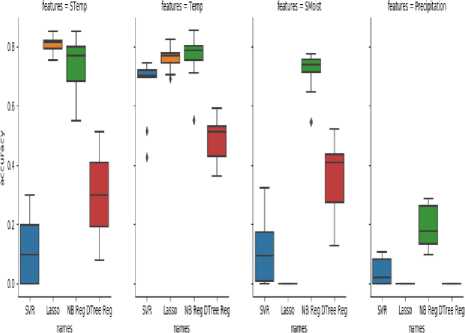
Fig.8. Prediction Accuracy for Weather and Soil Attributes Using SVR, Lasso, Naive-Bayes and Decision Tree Algorithms

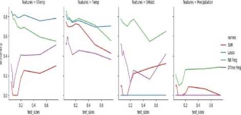
Fig.9. Accuracy V/s testing size for Weather and Soil Attributes Using SVR, Naive-Bayes, Lasso, and Decision Tree Algorithms

Fig.10 represents the NDVI prediction where the dataset has 380 samples in total and 180 samples of data have been taken as a base for training the dataset, the testing dataset consists of multiple samples which have been increased periodically. The sample size for every run varies which results in various accuracy scores from which the maximum score would be considered.

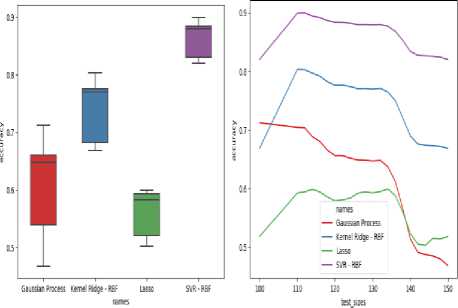
Fig.10. Box and Whisker and Line Plot for NDVI prediction

In Fig.10, SVR-RBF yields 89.97% accuracy for 112 samples of data in NDVI prediction. When we look at the entire range of accuracies and perform analysis, minimum accuracy obtained for SVR-RBF is 82.02% with 100 samples considered, and maximum accuracy obtained is 89.97% for 112 samples. When the median is considered for the entire range, the accuracy obtained is

87.98%. About 48% of the obtained accuracies lie below the median and 52% of the accuracies lie greater than the median, proving the algorithm implementation to be constant. After looking at the entire range of accuracies and performing analysis, minimum accuracy obtained for GPR is 46.86% with 150 samples considered, and maximum accuracy obtained is 71.231% for 100 samples. When the median is considered for the entire range, the accuracy obtained is 64.81%. About 48% of the obtained accuracies lie below the median and 52% of the accuracies lie greater than the median. After looking at the entire range of accuracies and performing analysis, minimum accuracy obtained for Kernel Ridge-RBF is 66.86% with 100 samples considered, and maximum accuracy obtained is 80.32% for 110 samples. When the median is considered for the entire range, the accuracy obtained is 77.05%. About 48% of the obtained accuracies lie below the median and 52% of the accuracies lie greater than the median. After looking at the entire range of accuracies and performing analysis, minimum accuracy obtained for Lasso Regression is 50.31% with 144 samples considered, and maximum accuracy obtained is 59.94% for 134 samples. When the median is considered for the entire range, the accuracy obtained is 58.36%. About 48% of the obtained accuracies lie below the median and 52% of the accuracies lie greater than the median. This algorithm has given a very low accurate prediction for NDVI. The line graph is shown in Fig.10 also depicts similar results for the applied algorithms for NDVI prediction. The fall and rise of accuracies for NDVI prediction can be observed in the above figure. These accuracies have also been plotted for exactly the same parameters as the Box and Whisker plot. The line graph depicts the trend in the accuracies for changing dataset sample sizes. Thus for the NDVI prediction, we can conclude that SVR-RBF is the best performing algorithm when compared to the other three algorithms and leads the pack with 89.97% of accuracy.

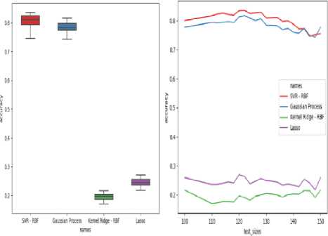
Fig.11. Box and Whisker and Line Plot for Crop prediction.

Fig.11 represents the crop prediction where the dataset has 380 samples in total, and 180 samples of data have been taken as base for training the dataset, the testing dataset consists of multiple slices which have been increased periodically, sample size for every run varies which results in various accuracy scores from which the maximum score would be considered. SVR-RBF yields 83.49% accuracy for 122 samples of data in crop prediction. After looking at the entire range of accuracies and performing analysis, minimum accuracy obtained for SVR-RBF is 74.53% with 146 samples considered, and maximum accuracy obtained is 83.49% for 122 samples. When the median is considered for the entire range, the accuracy obtained is 80.41%. About 40% of the obtained accuracies lie greater than the median, proving the algorithm implementation to be constant. After looking at the entire range of accuracies and performing analysis, minimum accuracy obtained for GPR is 74.29% with 148 samples considered, and maximum accuracy obtained is 81.71% for 122 samples. When the median is considered for the entire range, the accuracy obtained is 78.39%. About 48% of the obtained accuracies lie below the median and 52% of the accuracies lie greater than the median. After looking at the entire range of accuracies and performing analysis, minimum accuracy obtained for Kernel Ridge-RBF is 17.03% with 110 samples considered, and maximum accuracy obtained is 21.66% for 150 samples. When the median is considered for the entire range, the accuracy obtained is 19.68%. About 43% of the obtained accuracies lie below the median and 57% of the accuracies lie greater than the median. This algorithm has given the least accurate prediction for the crop. After looking at the entire range of accuracies and performing analysis, minimum accuracy obtained for Lasso Regression is 21.77% with 148 samples considered, and maximum accuracy obtained is 27.03% for 120 samples. When the median is considered for the entire range, the accuracy obtained is 24.41%. About 48% of the obtained accuracies lie below the median and 52% of the accuracies lie greater than the median. This algorithm has given a very low accurate prediction for the crop. The line graph also depicts similar results for the applied algorithms for crop prediction. The fall and rise of accuracies for crop prediction can be observed in Fig.11. These accuracies have also been plotted for exactly the same parameters as the Box and Whisker plot. The line graph depicts the trend in the accuracies for changing dataset sample sizes. Thus for the crop prediction, we can conclude that SVR-RBF is the best performing algorithm when compared to the other three algorithms and leads the pack with 83.46% of accuracy.

• VII.    Conclusion and Future Scope

Earlier researchers have worked on predicting sugarcane yield for small regions where weather conditions and sowing start times were the same. In this research, we have successfully modeled sugarcane yield prediction considering different sowing start period under different conditions in India region with an overall accuracy of 83.49%. We have also developed a model which can predict crop yield in real time by predicting weather conditions using time series forecasting and predicting NDVI using predicted weather parameters and using NDVI predicting real-time crop. We have achieved accuracy of 85.24% for Soil Temperature given by Lasso, 85.372% accuracy for Temperature given by Naive Bayes, accuracy for Soil Moisture is 77.46% given by Naive Bayes, accuracy for Precipitation is 28.69% given by Naive Bayes for weather and soil attribute prediction, 89.97% for NDVI forecasting and 83.49% for final yield prediction. In the future, we can consider predicting sugar-cane yield considering variable growth periods of 12 months and 18 months. Since SVR has emerged as a better algorithm, we can also use various Kernel functions to reduce noise in the dataset, to consider a better seasonal variation. We can also think of using ensemble learning methods and compare accuracy with SVR.