Supervised Online Adaptive Control of Inverted Pendulum System Using ADALINE Artificial Neural Network with Varying System Parameters and External Disturbance

Published Online July 2012 in MECS

The inverted pendulum problem is a classical example of an unstable nonlinear dynamic system. Therefore, much attention has been given to explore a better solution for it and further, to solve other similar control problems. Nonlinear system control now occupies an increasingly important position in the area of process control engineering as reflected by the tremendous increase in the number of research papers published in this area. Artificial neural network proved to be a useful tool in dealing with applications such as pattern recognition, signal processing, image processing and various complex controls and mapping problems etc. Neural networks have been applied successfully to identify and control of dynamic systems because of their learning capacity and ability to tolerate incorrect or noisy data [1]. The universal approximation capabilities of the multilayer perceptron make it a popular choice for modeling nonlinear systems and for implementing general-purpose nonlinear controllers. A conventional controller which is discussed in [2] is used to collect the training data to develop Neural Network controller for a inverted pendulum system. Multilayer neural network consists of single layer each for inputs and outputs and one or more hidden layers, each layer can have one or more no’s of neurons. The linking weights are updated by the back-propagation algorithm. It can control different systems through quick learning process and has perfect performances. Ni (1996) proposed a method for identification and control of nonlinear dynamic system a recurrent model was applied as identifier [3]. Gupata (1999) presented an improvement to back-propagation algorithm based on the use of an independent, adaptive learning rate parameter for each weight with adaptive nonlinear function [4]. LM algorithm is an effective optimization technique that can guide the weight optimization [5]. Neural network has been widely applied for state feedback controller design, nonlinear system control, nonlinear dynamical system identification, optimal control synthesis and three-dimensional medical image [6-10]. The ADALINE neural network is revisited and generalized in [11] by introducing a momentum term in the LMS learning algorithm. The momentum term helps to speed up the learning process and reduce the zigzag effect during convergence period of learning. This paper uses the regularized LM algorithm to offline train the connecting weights of neural network and for online training of ADALINE ANN LSM algorithm is used. The objective of this paper is to develop both online and offline neural network-based nonlinear controller for IP system and provide a rapid, reliable solution for the control algorithm.

II.    ADALINE Artificial Neural Network

ADALINE is one of the basic models used for data prediction. This method has not found much application to predict nonlinear system dynamics because it is slow in convergence therefore multiple ADALINE units are combined together and named as MADALINE in [11] to capture the dynamic behavior of the feedback control law and to control the IP system. A generalized (ADALINE) neural network, called GADALINE, for online identification of linear time varying systems which can be described by a discrete time model. GADALINE is a linear recurrent type of neural network. In such networks, the current system output is dependent on past outputs and on both the current and past inputs. So the GADALINE needs to have output feedback and to remember past input/output data. The author further generalizes the adaptive learning by adding a momentum term to the GADALINE weight adjustment. This momentum term is turned on only during convergence period and the GADALINE's learning curve is therefore smoothed by turning off the momentum once the learning error is within a given small number. The low computational complexity makes this method suitable for online system identification and real time adaptive control applications. Simulation results showed that GADALINE provides a much faster convergence speed and better tracking of control law than the generalized Radial Basis Function (GRBF) which is discussed in [12].The structure of an ADALINE is shown in Fig.1.

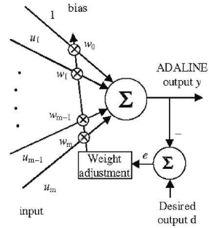
Fig.1. A single ADALINE unit

Widrow-Hoffs delta rule or Least Mean Square algorithm (LMS), is based on minimizing the error function,

Е(W)=1⁄2е2 (t)(4)

where t is the iteration index and e(t) is given by,

е(t)=d(t)-У(t)(5)

where the desired output d(t) at each iteration t is constant.

The weight adjustment is,

Δw(t)=туе (t)и(t)(6)

and

w(t + 1) = w(t)+Δw(t)(7)

or

w(t+1)=w(t)+туе (t)и(t)(8)

Here the learning-rate parameter is usually in the range of 0< Л <2. To speed up the convergence, a momentum term is added into the weight adjustment equation (6).

The new weight adjustment now becomes,

∆w=   ( t ) и ( t )+ a ∆w( t - 1)       (9)

Where 1 >  a ≥ 0 is a small non- negative number, to see the effect of the momentum, we can expand the equation starting from t = 0,

∆w(0) = Tje (0) и (0)

∆w(1) = Tje (1) и (1) + a ∆w (0)

=   (1) и (1) + a T)e (0) и (0)

∆w (2) = Tie (2) и (2) + a ∆w(1)

=   (2) и (2)+ arje (1) и (1)

+ a²rie (0) и (0)

If we consider the notation for inputs as u1-um , then the output y can be found by,

∆w( t )=U

∑

a^{£ T}e( t ) и ( t )

’ =∑

Remember e ( t ) и ( t ) is just – dE ( t )/ dw ( t ), then

=

Where u is the input vector and w is the weight vector,

∆w( t )=-и

∑

a^{£ T}dE ( т )/ dw ( т )

и =[ U_T U₂ …   ]т             (2)

W=[ W, W₂ …   ]т            (3)

So, we have an exponentially weighted time series. We can then make the following observations,

The GADALINE learning algorithm is based on the Widrow-Hoff rule with a momentum added to the weight adjustment stage. The implication on addition of the momentum term to learning algorithm is discussed in [11] as follows.

a) If the derivative dE ( t )/ dw ( t ) has opposite sign on consecutive iterations, the exponentially weighted sum ∆ w ( t ) reduces in magnitude, so the weight w ( t + 1) is adjusted by a small amount, which reduces the zigzag effect in weight adjustment.

• b) On the other hand, if the derivative дE ( t// d w (t) has same sign on consecutive iterations, the exponentially weighted sum Aw(t) grows in magnitude, so the weight w(t + 1) is adjusted by a large amount. The effect of the momentum term is to accelerate descent in steady downhill region.

Because of this added momentum term, the weight adjustment continues after convergence, that is, when even the magnitude of the error term e is small. For linear system identification purpose, these weights correspond to system parameters. It is desirable to keep these parameters fixed once convergence is seen. So we should turn off the momentum term after convergence is detected, say |e| < ε, ε > 0, is a small number. However, when the system parameters change at a later time, another convergence period will begin, and then it is better to turn the momentum back on.

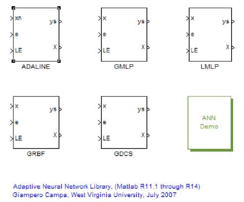
Fig.2. Adaptive neural network toolbox

GADALINE training is performed by presenting the training pattern set, a sequence of input-output pairs. During training, each input pattern from the training set is presented to the GADALINE; the GADALINE computes its output y. This value and the target output from the training set are used to generate the error and the error is then used to adjust all the weights [11].

The step based training algorithm for an GADALINE is as follows:

Step1: Initialize the weights (non-zero i.e. some random small values are used). Set learning rate r] and momentum term a.

Step2: While stopping condition is false, do step 3-7.

Step3: For each bipolar training pair u: d , perform steps4-6.

Step4: Set activations of input units u_i=s_i , for i=1 to m .

Step5: Compute net input to output unit as:

’=2

w_tu_t = T^TW 1

Step 6: Update network weights, as:

w(t + 1/ = w(t) + T]e(t)u(t) + aAw(t - 1)

Step 7: Test for stopping condition.

The stopping condition may be when the weight change reaches small level or number of iterations etc [13].

This problem is solved by using an adaptive neural toolbox which is an add-on for MATLAB simulink [15]. This toolbox basically allows for online neural learning to occur. The block diagram of the toolbox is shown in Fig.2. This toolbox contains an ADALINE and RBF (Radial Basis Function) simulink blocks.

The inputs to each block are:

• x: The input vector to the neural network.

• e: The error between the real output and the network approximation.

LE: A logic signal that enables or disables the learning.

The outputs of each block are:

Ys: The value of the approximate function.

X:  All the “states” of the network, namely the weights and all the parameters that change during the learning process.

There is an interface for each block so that the user can set the network parameters such as learning rate, number of the neurons in each layer, etc.

A. Modeling of Inverted Pendulum and Controllers

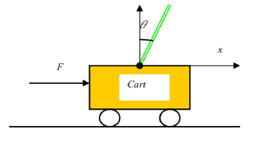
Fig.3. Inverted pendulum system sketch

The inverted pendulum system, as shown in Fig.4, is composed of a rigid pole and a cart on which the pole is hinged [14]. The cart moves on the rail track to its right or left, depending on the force exerted on the cart. The pole is hinged to the car through a frictionless free joint such that is has only one degree of freedom. The control goal is to balance the pole starting from nonzero conditions by supplying appropriate force to the cart. The displacement of the cart can be measured by a sensor installed on both sides of the rail track, and the angle signal can be measured by a coaxial angle sensor installed in the bearing which articulates the pendulum to the cart. On one side of the rail track a DC permanent magnetic direct torque motor is mounted which drives the cart to move on the rail track using a driving belt. When the cart moves left and right, torque act on the pendulum to keep the whole system in stable condition. Masked values of system plant parameters are used so that it can be easily varied to check the performance of the proposed controller with different system parameters. The cart mass is M, the pendulum mass is m, its length is 2L. The cart is restricted to move within a fixed range. The reference position for x is 0 meter, when cart is in the center of the rail track and for θ is π radians, when the pendulum is at a natural stable downward position.

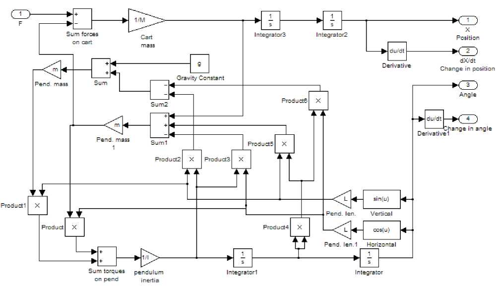
Fig.4. simulation model of nonlinear inverted pendulum system

• B.    Mathematical model of inverted pendulum

The dynamic equations of the system can be found with help of the Euler-Lagrange equation as in [2]:

(м+т ̈+ḃ+mL ̈cosО- mLṫ2 sin о)=F

(I+ ml?) ̈+mgL sin 6=-mL ̈cos9      (1)

Now by using the above equations the nonlinear model of IP system is developed in MATLAB simulink [15] which is shown in Fig.4.

• C.    Feedback control law for Inverted Pendulum System

To provide the supervised training data for the neural network controller we use the direct adaptive control technique described in [2]. Based on the equation (1) the following equations are a control law developed for the inverted pendulum controller. The first four equations (2-5) are entered into the main equation. The main equation (6) calculates the required force, u to keep the pendulum stable.

3
ℎ Y =	(2)
3
ℎ= 4 L	(3)
fi =   ( LstnSt ̇2 - 3 gsin 2 9 )	(4)
f2 =  + m (1-3 cos29 )	(5)

и= [ℎ i+ ki (0- 6(1)+k2ṫ+Cl (X- Xd)+C2̇]-

A                                          (6)

The following numeric values are used: M=1.096 Kg , m=0.109 Kg , L=0.25 m , g=9.81 m/s² , k 1 =25, k 2 =10, c 1 =1, c 2 =2.6 . Also xd = 0 meter and θd = 0 radian which are the desired position of the cart and angle of the pendulum respectively. A simulation model of the above control law was developed and is shown in Fig.5.

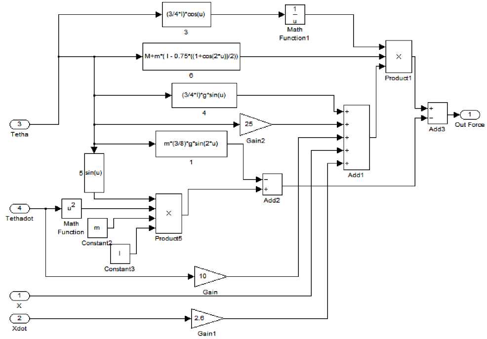
Fig.5. Simulink model of nonlinear control law

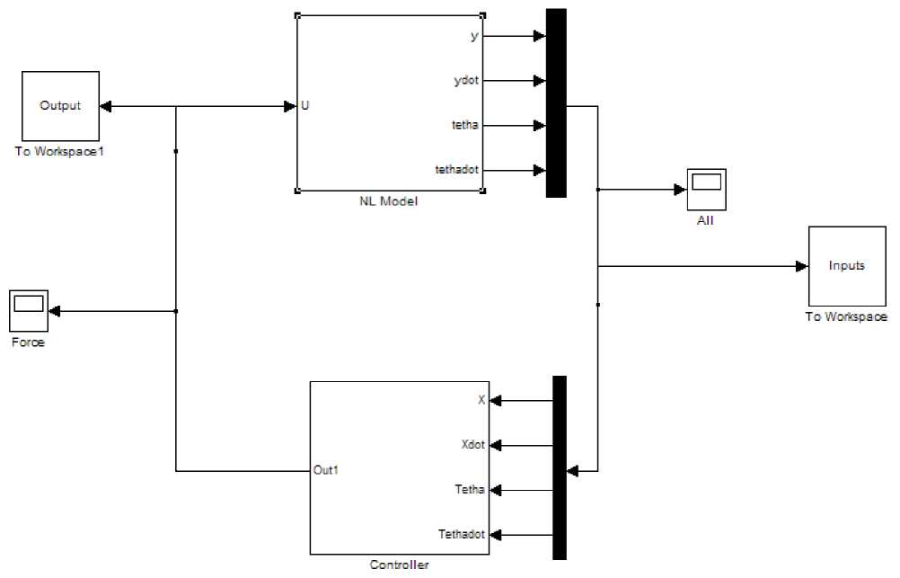
Fig.6.Simulink blocks of non-linear model of inverted pendulum and controller

• D.    Offline trained ANN Controller for Inverted pendulum

  The offline ANN has been trained by using the training data generated by the feedback control law from the setup shown in the Fig.6, the offline ANN training specification is given as: network type is feedforward, network training function is Levenberg-Marquardt algorithm (trainlm), input activation function sigmoid (tansig), output activation function is linear(purelin), no. of iterations (epochs) is 1500,

learning rate is 0.1, momentum control factor to avoid the problem of local minima is 0.1, no. o f neurons in input hidden and output layers are 4,13,1 respectively. After training the neural net with the above settings the simulation block has been generated using the command

Gensim (network_name, desired_sample_time) in the MATLAB command prompt. The simulation model of the trained neural network controller is shown in Fig.7.

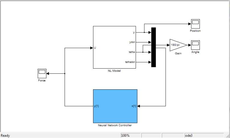
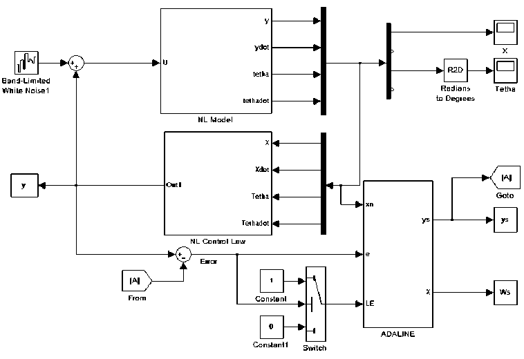
Fig.8 below shows the simulink setup of the adaptive learning. The error signal is equal to the output of the controller minus the output of the network. This signal is fed back into the GADALINE. The weights in the

GADALINE are updated using the steepest descent gradient, which minimizes the square error between measurements and estimates. The learning rate of the GADALINE is set to 0.1 and the sample rate to 0.01.

III.    SIMULATION Results and Analysis

The simulation results show the closed loop response of inverted pendulum with online and offline controller systems. The simulation time is 10 seconds for all simulations with fixed step size solver of sample time 0.01 second. Three experiments are performed to demonstrate the online adaptability and controlling ability of the proposed neural network controller for the inverted pendulum system under the application of initial condition, band-limited noise and for some parameter variations of the inverted pendulum system.

In the first experiment the initial parameters of the inverted pendulum system are listed as follows: x (0)=0.0 m , x(0) = 0.0m/s , 9 (0)=0.0 rad , 0(0) = 0.0rad/s These values are putted in the initial condition column of the integrator blocks of nonlinear inverted- pendulum model corresponding to cart position, cart-velocity, pendulum angle and pendulum angler velocity respectively. The disturbance is introduced externally in the form of band limited white noise with noise power 0.1 sample time 0.01 and seed value of {16}.

The simulation setup for the first experiment is shown in Fig.8 with ADALINE block parameters are as follows: 4- inputs (cart position, cart-velocity, pendulum angle, and pendulum angular velocity), 1-output (force on cart), 1.0- learning rate, 1e-6 -stabilizing factor, Inf –weight limiter, 0-initial condition, 0.01-sample time. The corresponding Simulink results are shown in Fig.9. The experiment result shows that the ADALINE ANN controller adapts its weights to respond similar to the desired value.

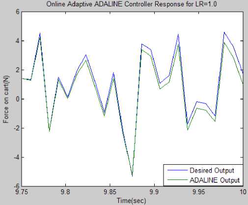
Fig.9 Simulation results of online adaptive ADALINE controller

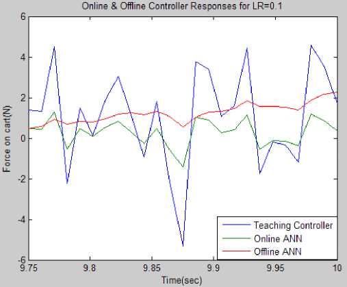
Fig.10 Simulation results for online and offline controllers

Now in second experiment the parameters are set to zero initial values as x(0)=0.0m, x(0) = 0.0m/s, 9(0)=0.0rad, 0(0) = 0.0rad/s, and the disturbance is introduced externally in the form of band limited white noise with noise power 0.1 sample time 0.01 and seed value of 16. The ADALINE block parameters are as follows:   4- inputs (cart position, cart-velocity, pendulum angle, and pendulum angular velocity), 1-output (force on cart), 0.1- learning rate, 1e-6 - stabilizing factor, Inf –weight limiter, 0-initial condition, 0.01-sample time. The simulation setup for the second experiment is shown in Fig.8 and results are shown in Fig.10 and Fig.11 from the results in Fig.10 it is clear that for learning rate of 0.1 online ANN responds better than the offline trained ANN and the performance of online trained ANN can be further improved if we increase the learning rate which is shown in Fig.11 that for learning rate of 0.5 and 1.0 the adaptive ADALINE ANN controllers output is very close to the reference controller.

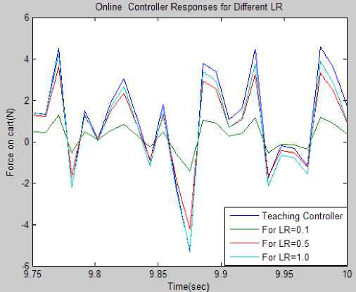
Fig.11. Simulation results of ADALINE for different learning rates

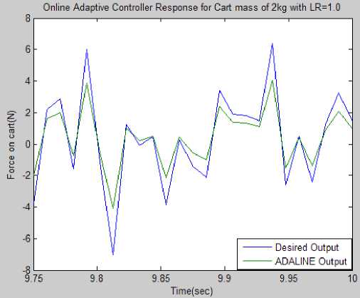
Fig.12. Simulation results for changed cart mass of 2kg with simulation time 10 seconds

Finally in third experiment the parameters are set to initial values given as x (0)=0.0 m, x(0) = 0.0m/s, 6 (0)=0.0 rad, 0(0) = 0.0rad/s . In this experiment the value of cart mass M is increased nearly 100% and it is changed to 2 kg the simulation setup is same as that of first experiment except that now the cart mass is 2 kg. The disturbance is introduced externally in the form of band limited white noise with noise power 0.1 sample time 0.01 and seed value of {16}. The ADALINE block parameters are as follows: 4- inputs (cart position, cartvelocity, pendulum angle, and pendulum angular velocity), 1-output (force on cart), 1.0- learning rate, 1e-6 -stabilizing factor, Inf –weight limiter, 0-initial condition, 0.01-sample time. Simulation result for the changed mass of cart is shown in Fig.12. Results shows that control action by online adaptive ADALINE is similar to the teaching controller and it can be improved if we increase the simulation time 20 sec as shown in the Fig.13, the ADALINE output is now more close to reference output.

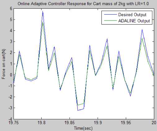
Fig.13. Simulation results for changed cart mass of 2kg with simulation time 20 seconds

IV.    Conclusion

This paper introduced Online and offline artificial neural networks to control the inverted pendulum system. The advantage of neural network is its nonlinear nature to predict the nonlinearity in the system. To generate supervised data to train the ANN controller the IP system is stabilized by the control law. The data generated is used train both kind of neural network controllers so that they can mimic the output of control law by optimizing the linking weights and bias values. These trained neural network controllers are tested in MATLAB Simulink with nonlinear inverted pendulum model. Simulation results show that both online and offline ANN controller stabilizes the IP system under uncertain parameters and it is also able to handle external disturbances. ADALINE ANN proved to be very fast and accurate in online prediction and control. Based on the simulation results proposed ANN controllers can be used to control the real time IP system.