Supervised support vector machine in predicting foreign exchange trading

Published Online September 2018 in MECS

Machine learning methods using computer science play important role in many areas such as business decision making, handling or monitoring factory chain, predicting or forecasting stock, and so on. The main task in machine learning is to teach computer systems abilities of learning to classify or cluster from given data set. In business area, machine learning especially supervised learning methods can effectively help users to analyze the big data collected from alternative resources to extract useful knowledge. For example, given currencies exchanging rate data from online transaction, supervised learning can predict the rise or fall in short or long period based on learning from historical data.

Supervised learning is one of machine learning methods to automatically build a predictive function f: x^ y that maps x to a prediction y [13]. This means the given data set has a structure of {%, y} where x can be seen as the raw data and y will be the target label. The task of supervised learning technique is to predict the expected output based on the historical data.

Almost supervised learning techniques are used for classification and regression tasks. It is also so-called Intelligent Systems as it has been developed based on Artificial Intelligence system such as Logical/Symbolic techniques, Perceptron-based techniques and Statistics (Bayesian Networks, Instance-based techniques) [22].

The task is called classification if the target variable (y) is categorical (nominal or discrete) and called regression when y is continuous (real-valued) [13]. For simple, many classification problems are treated as a binary classification task. On the other words, the output can be seen as binary attribute.

Support Vector Machines (SVMs) are the supervised machine learning techniques [26]. SVMs revolve around the notion of a “margin”—either side of a hyperplane that separates two data classes. Maximizing the margin and thereby creating the largest possible distance between the separating hyper-plane and the instances on either side of it has been proven to reduce an upper bound on the expected generalization error [22]. Therefore, SVMs can be used to solve binary problems such as predicting Foreign Exchange (Forex) trend (Uptrend or Downtrend) based on historical data of Open", "Close", "Low" and "High" in alternative time periods.

This paper has been organized in 5 sections. Section 1 shows the introduction of machine learning technique and Forex problem. The related works can be seen in section 2. Detail support vector machine (SVM) method and Forex problem are introduced in section 3. The section 3 also shows the detail deployment of Expert Advisor (Robotics) with using SVM model for FoRex transactions with demo account. This is considered as a novel contribution for the paper as not many previous researches have done before. Section 4 shows the experiments of using support vector machine model in predicting the Forex trend and their results. The results of using Robotics with and without SVM for FoRex transactions also are represented in this section in order to show the advantage of using SVM model. The conclusion is represented in section 5.

• II.    Related Works

  The Forex prediction problems have usually be seen as the binary classification ones because the expected output is one of either rise or fall foreign currencies rate trends. Box and Jenkins' AutoRegressive Integrated Moving Average (ARIMA) technique has been widely used for time series forecasting. However, ARIMA is a general unvaried model and it is developed based on the assumption that the time series being forecasted are linear and stationary [1]. According to [1], exchange rates prediction is one of the most challenging applications of modern time series forecasting. This is because of the inherently noisy or non-stationary rates [9]. In this case, the historical data is the major factor during the prediction process. The researches in [1, 8- 9] have used Radial Basic Function (RBF) and Multilayer Perceptron Network (MLP) models for the FoRex classification whereas the one in [18] used gene models. The research in [1] has used a data set of 1825 instances including a training of 1600 and testing set of 225 observations. It seems that there was a small volume of historical data set in order to train the model. The ANN model included multilayer perceptron network with a structure of 3 input nodes (price, weight, and fluctuation of prices), 2 hidden nodes and 1 output node (changed or unchanged). The model weights were calculated by gene algorithm with 8 genes in alternative chromosomes. The disadvantage of this model is simple as well as using of small data set for the experiments so that the quick regression of model might be mistaken. The mining data in Rumania stock using neural network models for price prediction also can be seen in [6]. The neural network such as MLP (multilayer perceptron) is not only successful in classifying of electroencephalogram (EEG) [12, 21] but also it has been used to predict the future price of stock code in financial field. The results have shown the advantages of using supervised learning techniques in predicting classification problems. Other research on predicting trends in stock market can be seen in [3, 5, 23, 28-29]. Their researches have reported using artificial neural networks or decision tree models. However, many of these papers reported that they are able to work in realtime settings and according to [19], there remains a lack of published research using high frequency data. For example, in [23], neural network results shown quite good accuracy (less than 5%) in short-term prediction of exchange rates (EUR/USD, GBP/USD and USD/JPY) in daily, monthly and quarterly. However, the size for the training, testing sets were very small (less than 83 observations in total). Therefore, the results might not be the general representative solution for FoRex prediction problems or the quick regression might be taken. Moreover, the research in [23] used one-step mode in neural network method. This simple mode might not deal with complicated FoRex problems such as many input variables, big size of transactions etc.

Finding solution in financial problem also has been interested in [11]. In there, the stochastic differential equation, which is usually used determining boundary in financial problems such as asset pricing or Asian option to buy the asset at the future time, etc., has been used with Euler-Maruyama method. However, the assumption of linear equation seem to be hard to apply in non-linear hyperplan (non-linear dataset) in FoRex predicting problems.

Many publications have shown that SVMs were extended to solve nonlinear regression estimation problems and have been successfully used to solve forecasting or classification problems in various fields [16, 24, 25]. However, according to [14], there is not many studies for the application of SVM in financial time-series forecasting, although SVM has some advantages [7, 17]. Recently, the research in [2] has shown an integration of Genetic Algorithms and Support Vector Machine to trade in the FoRex market. In there, SVM is used to identify and classify the market and Genetic Algorithm is used to optimize the trading rules which are based on the best SVM classified indicators.

For above reasons, in this paper, SVM model is chosen to predict the rise or fall of currencies rates in FoRex market. Moreover, it is installed into Expert Advisor (Robotics) for making transactions. Another reason of choosing SVM is because of no parameters to tune except the upper bound C [10], and SVM avoids over-fitting problems like other Artificial Neural Networks models [13].

• III.    Supervised Support Vector Machines and Foreign Exchange Prediction

• A.    Supervised Support Vector Machine

Support Vector Machines (SVMs) are so-called as linear or non-linear SVMs depending on linear or nonlinear hyperplane lines separating the training data set. In linear hyperplane, the formula of linear line as follows:

H: w. x + b = 0.

Assume that y_t E {+1, -1} , i = 1, n . y , is labelled output class. Then outputs will be separated by:

1 if w.X ( + b > 0

.-1 if w.X[ + b < 0

y‘=(

The hyperplane H has maximum margins to classes. That means SVMs need to build two others lines as: H₁: w. x + b = 1 ; and H 2 :w.x + b = —1 where there is no existing X [ in H₁ and H 2 , and the margin between in H₁ and H 2 is maximum. If the margin is maximum, there are some data points having positive labels and negative labels in the line of Щ, and H 2 respectively. These data points can be called as support vectors in hyperplane of H which can separates the data into two regions of positive and negative labels.

The distance of x in H₁ and H 2 to H can be calculated as:

|wz+b±1| _  1

Ml = M

Therefore, the margin can be calculated as:    , where

Hw||

^{+ w} 2 + — + ^w 2 .

/(x) = sign(w.x + b)

= sign

= sign

V t=1      V )

(/

)

On the other words, the maximum margin will be referred to minimum of ^                       (2)

with the subject to: y_t(w. x_t + b) > 1,i = 1,2.. n.

To sum up, the problem is referred to min-||w||2 where yt. (w.xt + b) > 1,i = 1,2,..n w,b 2

This is a quadratic convex optimization problem.

The problem in (3) can be replaced as dual problem as follows:

By using Lagrange factors a = (a 1 ,a₂, ..,a_n) > 0 , we have:

. z x ( 1 rm x > 0 Where: sign(x) = {     ,.

I —1 voi x < 0

For non- linear hyperplane in non-linear training data set, a solution for the inseparability problem is mapping data onto a higher dimensional space (the transformed feature space), where a linear hyperplane can be used there.

Ф: K^d ^ №^d ' x ^ Ф(x)

The Equation of (7) will be:

n     nn

^—D = E a i - 7 E E a i ^ a j ■ ^yi'^yj ^ф x i ^{) ф} x j )    ⁽⁸⁾

i = 1         2 i = 1   j = 1

n

n

t=1

max „ £(w, b, a)

t=1

With constrains as:

n

7— = w — У a y, x, = 0          (5)

dw                      ii ■ i i=1

n

= ^— E ay ^{0          (6)}

i = 1

Where Ф(x_t).Ф(x₇•) = k(x_t,x_j') is so-called as “kernel function” [4], this kernel function is used to map new points into the feature space for classification whenever a hyperplane has been created.

In some cases, SVM may not be able to find any separating hyperplane as if the data contains misclassified instances. In this situation, SVM used a soft margin that accepts some misclassifications of the training instances [15].

In other words, the D set might contain noisy data. At this time, the constraint of no existing data point between H 1 and H₂ is not guaranteed. However, we can put positive variables of ^_t to change the conditions of H 1 and H₂ as:

And a > 0.

From (5) and (6) we have:

Therefore, the expression of —(w, b, a) will be: n     nn

^— _D = ^—(w^,b,a) = у a -~ EE a- a j ■ y - y j x^ ^xj ⁽⁷⁾

i = 1         ² i = 1 j = 1

With a = (a 1 , a₂, ..., a_n) and given b we have:

For each x E №d will be classified by:

wx_t + b > 1 — f_t   where y_t = +1

wx_t + b < —1 + f_t   vwhere y_t = —1

^t>0,              i = 1,2,...,n

We define a coefficient of fine C (positive value) to the objective function for the noisy data points as:

^min w,b^ l 2 ^w 2 + C.I у ^ i )  )

Basically, m equals as 1, therefore, the optimization problem can be seen as:

min w.b.f ( 1 w² + C. £ⁿ =1 ^ t )           (10)

With the constraints:

yt(w.xt + 6) + ft — 1 > 0, i = 1,2, .^,n ft>0,                    i = 1,2n

In Dual problem there are no variables f_t , the constraints a_t have a super limitation of C. We have:

All above cases will be used to recalculate the Lagrange values during training models process.

Training SVM models algorithm

The popular algorithm used for SVM models is Sequential minimal optimization – SMO [20]. The SMO solved the dual optimization problem as:

n     nn тахЛ = У a-y^S aiajyiyjxv xj i=1        2 i=1 j=1

max£fl

a

n

^

a ,

i=1

n   n

— Z^^Wiy/i'x i=1 7=1

With constrains:

with conditions 0 < a_t< C, Vi and E n= ₁a_ty_t = 0.

n

0 <  a t < C and ^ a t y t = 0 t=i

Karush-Kuhn-Tucker (KKT) conditions [27]

The condition of existing optimum optimization problem or dual problem as

values

for

n

= w — У a,- y, x, = 0

aw                      11■ i i=1

(12a)

SMO algorithm

Optimality Algorithm

Input: Training data, parameter settings

Output: a t as optimal

Optimality =0, and a , = 0

Repeat the following steps until reaching optimality

Step1 : Choose an adequate working set

Step 2 : Calculate new a , corresponding to QP subproblem

Step 3 : Update a ,

Step 4 : Check a stopping criterion for optimality.

n

^ = — У a_ty_t =0

аь                i i =1

(12b)

Assume that E (x, y) is prediction error for each pair of (x,y). Therefore,

-= 0 a<

(12c)

n

E(x,y) = ^

t=i

atytxt.x + 6

— y.

at(yt(w.xt + 6) + ft — 1) = 0, i = 1,2,,„,n

(12d)

(12e)

Depending on a_t E [0, C], we have:

• 1.    If a_t = 0 then ^_t = C — a_t = C > 0.

• 2.    If 0 < a_t< C then from (12d) we have:

• 3.    If a_t = C then from (12d) we have: y_t(w.x_t +

From (12e) we have f_t = 0.

Therefore:

y_t(w. x_t + 6) — 1 > 0.

y t (w.^ t + 6) + f t — 1=0.

Moreover, Д = C — at > 0 so ft = 0.

Therefore: yt(w. xt + 6) — 1 = 0.

• 6)    + f_t — 1 = 0.

Moreover, Д = C — at = 0 so ft > 0.

Therefore: yt(w. xt + 6) — 1 < 0.

According to [20], the selection of at, a;- will be performed in two heuristic loops so that |Et — Ej will be maximum. The Lagrange multipliers at are used in the process to select a at so that 0 < at < C and it is not satisfied Karush-Kuhn-Tucker conditions [27], and a;-(0 < a;- < C ) so that |Et — E;-1 will be maximum.

• B.    Foreign Exchange Prediction

The Forex market can be seen as a special one in financial markets with its characteristics of high benefits, maintaining capital in the case of inflation, and its transaction can be performed all the time at any location in the world. The investors can buy/sell the pairs of money such as EURUSD (Euro vs US Dollar), USDJPY (US Dollar vs Japanese Yen), GBPUSD (Great Britain Pound vs US Dollar) etc. to get benefits from different exchange rates between these pairs. In general, the following parameters define the trend of up or down of the rates:

• •    Target Profit (TP): is positive to indicate the target profit.

• •    Stop Loss (SL): is positive number to show that the loss is acceptable.

• •    Time Trend Detection (T): is positive to indicate the forward time starting from current point.

Therefore, given the current rate of (P), the outputs of prediction as:

• •    The trend of exchange rate is up if the rate is increased in term of (P+TP) instead of decreasing an amount of (P-SL) in the duration of T.

• •    The trend of exchange rate is down if the rate is decreased in term of (P-TP) instead of increasing an amount of P+SL in the duration of T.

The parameters of SL, TP are used with unit of “PIP” (to measure the profit or loss in the market).

Frame work of FOREX transaction

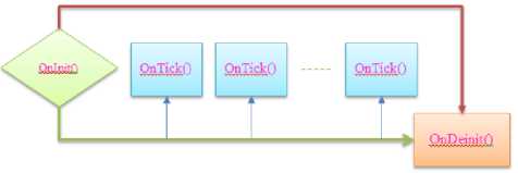
Fig.1. Frame works for Robotics in FoRex Transaction.

int OnlnitO

//Robotics initializations such as checking market information (minLot, maxLot, etc.), Pip,StopLoss, TakeProfit, Using SVM model or not, etc.

//return INIT_FAILED or INIT_SUCCEEDED return (INIT_SUCCEEDED) ;

void OnTick()

(

//Manage the Open, Close current demands ManagerOpenedPosition() ;

//Analyse the history data to predict of opening or closing

Checksignal(...);

Processsignal(...);

//Repeat until there is no change in the active FoRex pair.

void OnDeinit(const int reason) (

//Release memory for Robotics

• Fig.2. Initial Setting for Robotics Transaction.

The robotics performs transactions by using OnInit() function. If any change of current money pair has happened, OnTick() function will be performed to manage the opened or close demands as well as analyse the history of demands. If SVM model is used, the SVM models with alternative kernel functions and their parameters such as number of support vectors, C, γ , etc. will be used (see Fig. 3a, Fig. 3b).

The Ontick () function will be used iteratively until end of user transaction session time. At this time, the OnDeinit() will be used to release the robotics.

double SVM: :KernelFunc(int idx, double binVector [] ) ( double s = 0.0;

int d = MathMin(nDim, Arraysize(inVector));

int i;

switch (eKernel) (

// Gaussian RBF case klGsRBF:

//calculate SupportVectors for (i = 0; i < d; 1++)

s -= (Supportvectors[idx] [i]-inVector[i])*(Supportvectors[idx][i]-inVector[i]);

• return MathExp(-gamma * s);

  //Polynomial

case klPolynomi al:

// calculate Supportvectors for (i = 0; i < d; i++)

s -= Supportvectors[idx][i] * inVector[i];

return MathExp(MathLog(coeflin * s

• - coefconst) * poly_Degree);

  //Sigmoid Tanhyperbolic case klTanh:

  // calculate supportvectors for (i = 0; i < d; i++)

s -= Supportvectors[idx][i] * inVector[i];

return Tanh(coeflin * s + coefconst);

2________________________________

Fig.3a. SVM code installed in Robotics transaction.

double SVM::RealPredict(double sinVector[]) { double out = 0;

int i;

//Linear model if (eKernel = klLinear) ( int d = MathMin(nDim, Arraysize(inVector)) ;

//Calculate w * inVector for (i = 0; i < d; i—) out += w[i] * inVector[i];

//Nonlinear model else

{ for (i = 0; i < nSupportVector; i—) out -= alpha[i] * outs[i] * KernelFunc(i, inVector);

return (out - b);

}

Fig.3b. SVM code installed in Robotics transaction.

• IV.    Experiments

• A.    Data Configuration and Model preparation

Data

The FoRex data is collected by using MetaTrader 4 [30] to download from 01/01/2013 to 30/09/2016. In this paper, the pair of EUR/USD has been selected as it is very popular one in the market. The training data set D included the instances in a period of 01/01/2013 to 31/12/2015, and the test data set D’ contained the instances in a period 1/01/2016 to 30/09/2016.

Features

The selection of experimental features is effected to the model results. In this paper, the features are selected basing on the objectives of profits about 10 – 15 Pips for each transaction. The observed exchange rates are the "Open", "Close", "Low" and "High" for the candles in the window time of M1 (1 minute), M5 (5 minutes), M15 (15 minutes), H1 (1 hour) and D1 (1 day). The features are also based on the RSI (Relative Strengh Index), MA (Moving Average), Bollinger (Bollinger Bands), and Custom Indicators. The features are selected in the given data set can be seen in Table 1.

Table 1. 137 Selected Feature

Feature#	Data	N0	Note
#1-16	O, H, L, C on Timeframe M1	16	4 values x 4 candlesticks
#17-32	O, H, L, C on Timeframe M5	16	4 values x 4 candlesticks
#33-44	O, H, L, C on Timeframe M15	12	4 values x 3 candlesticks
#45-56	O, H, L, C on Timeframe H1	12	4 values x 3 candlesticks
#57-72	O, H, L, C on Timeframe D1	16	4 values x 4 candlesticks
#73-77	Time data	5	Data Attributes
#78-81	RSI(7) on Timeframe M5, M15	4	1 values x 4 Timeframe
#82-85	RSI(14) on Timeframe M5, M15	4	1 values x 4 Timeframe
#86-101	MA(9), MA(12), MA(100), MA(200)	16	4 values x 4 Timeframe
#102-113	Custom Indicator	12	4 PAX + 8 MKC
#114-119	Bollinger Bands	6	3 Lines x 2 Timeframe
#120-125	Average True Range	6	2 values x 3 Timeframe
#126-137	Highest, Lowest M1, M5	12	4 values x 3 Timeframe

Model configurations

The machine learning technique in the experiments is SVM model. Its model is used with alternative of Gaussian RBF, and Polynomial kernel functions. In detail, the model parameters are:

Hx-yH2

• •    RBF:     k(x,y) = e 20   = e ^{yHx yH}     with

Y E [0; 5]

• •    Polynomial:  k(x,y) = (x.y + 9)^d, 9 E K, d E N *

with d= 2,3,4 and 9 E [0; 1].

• •    The parameter of C has been used with C E [1; 10].

According [7] the upper bound C and the kernel parameter in kernel functions play an important role in the performance of SVMs. Therefore, after many performed experiments, the parameters have been used are follows as if they produce acceptable results.

• •    RBF: y E [1; 2] .

• •    Polynomial: d = 3 and 9 = 1.

• •    The parameter of C E [1; 2]

Table 2. Experimental Model Configurations

Models	Poly1	Poly2	Poly3	GsRBF1	GsRBF2	GSRBF3
C	1.0	1.0	1.0	2.0	1.0	2.0
Kernel	Poly	Poly	Poly	RBF	RBF	RBF
Parameters	Power 2	Power 3	Power 3	γ =5.0	γ =4.0	γ =5.0
No of vectors	3000	3000	2000	3000	4500	5000

• B.    Results

The data is used with the cross validation method. The D data set is divided in to Dpos (positive output); and Dneg (negative output). They are split to DpOS' ^pos, ■” , ^pos        ^l 6 p , ^l 6 p ,   , ^l 6 p           ( sub-sets has -|Bpos/n6p| samples. D_Test will be each sub-set and k-1 remaining sub-sets will be used for D_Train. In this paper experiment, k is chosen of 5. The results can be seen in Table 3 and Table 4 for 6 above models. The Accuracy Rate, Precision of Positive, Negative, Micro-Average and Macro-Average results are used to compare the performance between alternative models.

Table 3. RBF Configuration Models Results

Kernel: Gaussian RBF Features: 137		GsRBF1		GsRBF2		GSRBF3
		D_Train	D_Test	D_Train	D_Test	D_Train	D_Test
Accurate		82.41%	58.11%	86.08%	58.57%	87.28%	58.36%
Precisio-n	Positive	81.87%	57.61%	85.67%	57.78%	86.83%	57.59%
	Negative	82.96%	58.57%	86.50%	59.38%	87.75%	59.13%
	Micro-Average	82.41%	58.11%	86.08%	58.57%	87.28%	58.36%
	Macro-Average	82.42%	58.09%	86.09%	58.58%	87.29%	58.36%

Table 4. Poly Configuration Models Results

Kernel: Polynomial Features: 137		Poly1		Poly2		Poly3
		D_Train	D_Test	D_Train	D_Test	D_Train	D_Test
Accurate		76.78%	74.20%	82.46%	74.67%	82.52%	74.60%
Precisio-n	Positive	76.38%	74.69%	82.98%	78.40%	83.07%	78.50%
	Negative	77.19%	73.76%	81.95%	71.95%	81.98%	71.80%
	Micro-Average	76.78%	74.20%	82.46%	74.67%	82.52%	74.60%
	Macro-Average	76.78%	74.22%	82.47%	75.18%	82.53%	75.15%

• C.    Discussions

Table 3 and Table 4 show the results of alternative models using alternative kernel functions of Gaussian RBF and Polynomial respectively. The results in Table 3 show that the performance of positive and negative prediction for Test sets has big gap compared to the Training sets (about 53% and 82.5 % respectively). In contrast, there is a little different between performance rates of the training and testing in Table 4.

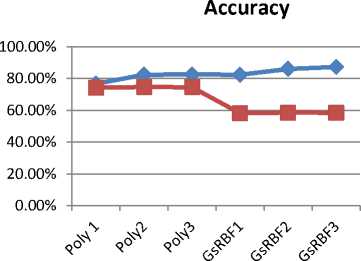
The accuracy rates taken from two kernel functions of

Gaussian RBF and Polynomial are represented in the chart to show the high performance of the use of Polynomial one in general. In Polynomial functions group (Poly1, Poly2, Poly3), there is no difference of accuracy rates for the Test sets (about 74.5%) whereas Poly2 and Poly 3 models have better results for the training set (82.5%). These results show that the use of C=1, polynomial power of 3 and alternative support vectors (see in Table 2) does not change the experiment performance.

D_train

D_Test

Fig.4. Accuracy rates of Experimental Model Configurations

• D.    Expert Advisor in FoRex Transactions

For comparison, the experiment of Robotics (expert advisor) without using support of SVM also has been used. The conditions for experiments as follows:

• •    Use Backtest function

• •    Broker: ICMarkets

• •    Currency pair: EUR/USD

• •    Time: 9 months

• •    Initial Margin: 1000USD

• •    Margin Level: 1:500

• •    Spread: 0.8 – 1.0 pip

• •   Commission: 7USD

The experiment results can be seen in Fig. 5 whereas the details of indicators’ results of No_SVM and SVM used for EA can be seen in Table 5.

Table 5 shows the advantage of using SVM in the transaction Robotics, in overall. For example, the Volume using SVM is a half of No_SVM (96 and 189 respectively) whereas the Profit rate is triple (3.03) compared to 0.77. The Fair Drawdown in the use of SVM is a little bit high (34.69%). But it is still a half of the one using without SVM implementation.

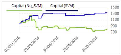
Fig.5. Experiment Results.

Table 5. Indicators’ Results

Index	Indicators	No_SVM		SVM
1	Net Profits		-210.46		337.94
2	Gross Profits		718.37		504.7
3	Gross Loss		-928.83		-166.77
4	Profit rate		0.77		3.03
5	Growth		-21.0%		33.8%
6	Average Growth (month)		-2.59%		3.29%
7	Strict Drawdown		371.72		151.5
8	Fair Drawdown	645.36	50.67%	450.67	34.69%
9	Volume		189		96
10	Profit Transactions	147	77.8%	85	88.5%
11	Loss Transactions	42	22.2%	11	11.5%
12	Ask Profit Transactions	111	91.0%	71	100.0%
13	Bid Profit Transactions	78	59.0%	25	56.0%

• V.    Conclusions

  The supervised machine learning technique such as support vector machine can help to solve the FoRex problem as it can be represented in binary classification task. The power of using artificial intelligence in learning models helps to deal with a huge, complex and time series data to extract knowledge for users’ purpose. For example, in this paper, an amount of experimental data set of more than 13500 instances has been performed. By using Gaussian and Polynomial kernel functions, the alternative models with alternative parameters have been performed. The results of using Polynomial Kernel have shown the better results compared to the models using Gaussian in general. To show the advantage of using SVM in the actual

The Robotics transaction in this paper is used with demo account, therefore, further research will focus on continuing to use transactional Robotics in the real foreign exchange market