Supplier Segmentation using Fuzzy Linguistic Preference Relations and Fuzzy Clustering

Автор: Pegah Sagheb Haghighi, Mahmoud Moradi, Maziar Salahi

Журнал: International Journal of Intelligent Systems and Applications(IJISA) @ijisa

Статья в выпуске: 5 vol.6, 2014 года.

Бесплатный доступ

In an environment characterized by its competitiveness, managing and monitoring relationships with suppliers are of the essence. Supplier management includes supplier segmentation. Existing literature demonstrates that suppliers are mostly segmented by computing their aggregated scores, without taking each supplier’s criterion value into account. The principle aim of this paper is to propose a supplier segmentation method that compares each supplier’s criterion value with exactly the same criterion of other suppliers. The Fuzzy Linguistic Preference Relations (LinPreRa) based Analytic Hierarchy Process (AHP) is first used to find the weight of each criterion. Then, Fuzzy c-means algorithm is employed to cluster suppliers based on their membership degrees. The obtained results show that the proposed method enhances the quality of the previous findings.

Еще

Supply Chain Management (SCM), Supplier Segmentation, Fuzzy Set, Fuzzy Linguistic Preference Relations, Fuzzy C-Means

Короткий адрес: https://sciup.org/15010560

IDR: 15010560

Текст научной статьи Supplier Segmentation using Fuzzy Linguistic Preference Relations and Fuzzy Clustering

Published Online April 2014 in MECS

Supply chain management is a process which consists of two or more work areas. These work areas include obtaining raw materials, transforming the raw materials into intermediate and finished goods, and finally distributing them to end consumers. Given the fact that firms are becoming more dependent on their suppliers [1-2], supplier management has garnered an increased attention from both academic fields and supply chain managers.Therefore, managing suppliers can strengthen firm’s competitive position in the marketplace by reducing transaction cost and increasing firm’s capabilities to adapt to unforeseen circumstances by finding perfect solutions [3].

Supplier selection and segmentation are prerequisites for supplier relationship management (SRM) [4]. Supplier selection is the process of choosing suppliers based on a number of criteria that are compatible with the company’s goals [5]. As a step between supplier selectionand supplier relationship management, supplier segmentation is the classification of similar suppliers in one group [2, 9]. While supplier segmentation is still in its infancy, many researches to date has been conducted on supplier selection using methodologies and techniques from diverse fields such as mathematical programming methods, artificial intelligence, and statistical techniques [6]. For a comprehensive review of the methods, one may refer to [7-8].

The term “supplier segmentation” was first introduced by Parasuraman [10] in 1980, but the variables required for segmenting suppliers were not specified. In 1983, however, Kraljic [11] proposed an approach with two dimensions by pre-specifying the segmentation variables: profit impact and supply risk. Although after Kraljic several two dimensional methods have been proposed [12-14] many of the important segmentation variables were neglected. Recently, Rezaei and Ortt [9] have established a list of variables and proposed a framework formed from two overarching dimensions: supplier capabilities and supplier willingness. Based on these two dimensions, they defined supplier segmentation as “the identification of the capabilities and willingness of suppliers by a particular buyer in order for the buyer to engage in a strategic and effective partnership with suppliers with regard to a set of evolving business functions and activities in the supply chain management”. The authors in [9] have applied fuzzy AHP as a multi-criteria decision making (MCDM) method to find the weights of capabilities and willingness criteria. Finally, based on each supplier’s aggregated score, the suppliers are divided into four segments. They have also adopted another approach to supplier segmentation which makes use of fuzzy logic

[2 ]. In their method, they designed two fuzzy rule-based systems so as to measure the aggregated score of suppliers’ capabilities and willingness. Lastly, they used the outputs of the two systems to segment the suppliers.

In this paper, we applied the same data used in [9], but instead of segmenting the suppliers based on their aggregated scores, fuzzy c-means clustering, a widely used algorithm in fuzzy clustering literature is employed.

Clustering techniques attempt to find grouping of the objects such that objects in a group are similar to each other and dissimilar to objects in other groups. The primary purpose of clustering is to find high-quality clusters with an increase in intra-cluster similarity and a decrease in inter-cluster similarity. Clustering is an unsupervised learning task and has been widely used in several domains such as machine learning, pattern recognition, and data mining.

The main contribution of this paper is to examine how fuzzy c-means method can handle supplier segmentation problem. The rest of the paper is organized as follows: Section 2 presents a description of the proposed method; Section 3 provides brief theoretical knowledge on Fuzzy AHP and Fuzzy c-means (FCM); Section 4 applies the proposed methodology to a real case. The final section discusses the findings and also leaves a space for future research.

and vagueness. Since this paper uses triangular fuzzy number (TFN), the following definition is presented [16]:

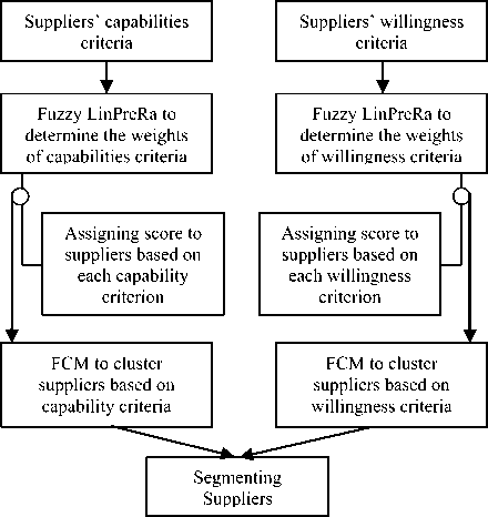
Fig. 1: Flowchart of supplier segmentation procedure

A fuzzy number N on R is defined to be a TFN if its membership function is:

II. Methodology

This section describes the steps used in our methodology for segmenting suppliers:

The first step is to identify a set of capabilities and willingness criteria in regard to the firm’s strategic aims and determine their weights using Fuzzy Linguistic Preference Relations based AHP. In the second step, a decision maker assigns a score to each supplier considering each capability and willingness criterion. The information obtained from the above steps is then combined to calculate the values of suppliers’ capabilities and willingness criteria. To cluster suppliers, Fuzzy c-means clustering (FCM) is applied twice- first for suppliers’ capabilities and then for suppliers’ willingness criteria. Finally, the output generated from clustering technique is used to segment suppliers. An overview of the procedure is also illustrated in Fig. 1.

Ha ( x ) =

---- l < x < m, m < x < u m -1

u - x otherwise

u - m

Where and are the lower and upper bounds of respectively, is the median value. The operational laws of two TFNs and are as follows:

Fuzzy number addition ⨁

A-lSAh = (Zpm^ti!) © (i^m^t^

III. Theoretical Knowledge

3.1. Fuzzy Set Theory

In this section, we introduce some definitions and notations pertinent to our proposed methodology:

Most of the phenomena we experience in daily life are imprecise or ambiguous by nature. Zadeh [15] introduced fuzzy set theory to overcome the uncertainty

Fuzzy number multiplication ⨂

^1®^: = (^i^i'^J ® (^'^2'ц;)

— Oi.X^l'TnlX Tn2-'lj,lXul)

Fuzzy number division (/)

Ai(/)A₂ = (li-m^ULX/) (l₂,m2,U2)

= (V^mt/m!,!»!/^

3. 2. Fuzzy Linguistic Preference Relations based AHP

Fuzzy AHP is the extension of the conventional AHP, which can solve imprecise hierarchical problems [16]. The main drawback to use fuzzy AHP method is that ensuring consistency in pair-wise comparison is difficult and it requires judgements for a level with n number of criteria [17]. In order to alleviate this problem, Wang and Chen [17] have developed fuzzy linguistic preference relations which reduces the number of pairwise comparison to П — 1 and results in consistent fuzzy ranking. Wang and Chen [17] defined the following statements to ensure the consistency of a fuzzy positive reciprocal matrix:

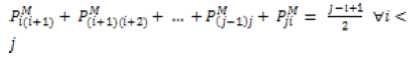
Proposition 1: For a fuzzy reciprocallinguistic preference relation, P = Fij with Pij e [0,1] ; verifies theadditive reciprocal, then, the following statements are equivalent.

approach used in different areas. Unlike hard clustering, in which the clusters are mutually exclusive, in FCM, each data object belongs to more than one cluster. To put it another way, each data object can belong to several groups with the degree specified by membership grades between 0 and 1 . Based on a defined similarity measures, data objects that are close to each other will be grouped in one cluster.

The primary goal of FCM is to minimize the following objective function:

^(ае) = 1и1М?Ь-С(Г (14)

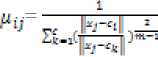
where F is the objective function, ^cxn is the membership matrix, ^ci is the cluster centre of the fuzzy group , fly is between 0 and 1, * is the Euclidean norm expressing the distance between i th cluster centre and ; th data object, and m is the weighting exponent which must be greater than one (m > 1).

Fuzzy clustering is done through an iterative optimization of the objective function in Eq. (14) with the update ofiUijandCf as follows:

Proof:See [17].

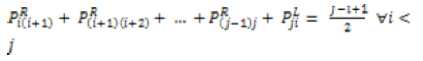
Proposition 2: For a reciprocal fuzzy linguistic preference relationP = Py = CPij.P*p”)to be consistent, verifies the additive consistency, then, the following statements must be equivalent.

In this method, there is an important constraint that must be imposed in the beginning of the algorithm, that is, the sum of the membership degrees of each data object to all clusters must be equal to one, Eq. (17)

^=L.^V =1, /6{1......c} (17)

A step by step procedure of the FCM algorithm is as follows:

FCM Algorithm:

Step 1: Set m>l;2 0; and choose an initial fuzzy c-partition matrix 17 .

Proof:See [17].

Step 2 : Calculate the fuzzy cluster centroid

CL for i = 1. ....c, using Eq. (16).

Step 3 : Apply Eq. (15) to update .^ij .

Step 4 : If f(U.c)<_£ , halt; otherwise go to step 2.

3.3. Fuzzy c_means

In the fuzzy clustering literature, fuzzy c-means (FCM) algorithm, first developed by Dunn [18] and further improved by Bezdek [19], is by far the most popular

IV. Experimental Results

In order to examine the proposed method, the suppliers’ data information found in [9] is adopted. This dataset is derived from a broiler company which has taken twelve criteria- six to measure suppliers’ capabilities (price, delivery, quality, reserve capacity, geographical location, and financial position) and six

others for suppliers’ willingness (commitment to quality, communication openness, reciprocal arrangement, willingness to share information, supplier’s effort in promoting JIT principles, and long term relationship. After applying fuzzy linguistic preference relations based AHP, the scores of capabilities and willingness criteria for each supplier are generated as the output (Tables 1-2).

After obtaining the criteria values for each supplier, FCM algorithm is employed for clustering process. The algorithm is applied twice - first, for evaluating suppliers’ capabilities and then for suppliers’ willingness. We have tested the result for с = 2 and с = 4, where с is the numbers of clusters. When the numbers of clusters are two, the suppliers are divided into High and Low levels, and when the numbers of clusters are four, they are divided into four levels (High, Medium High, Medium Low, and Low). The results are shown in (Tables 3-6).

To draw a distinction between the two clusters, the supplier with maximum membership degree in each cluster is found. Then, based on the aggregated score of the suppliers holding the maximum membership degree, the clusters are labelled. For instance, in the first cluster, supplier 11 is recognized to hold the highest membership degree and in the second, supplier 9 and10 . Their aggregated scores are then computed and compared. Since, the aggregated score of supplier 11 is greater than supplier 9 or 10 , cluster one is labelled as “High”, and cluster two as “Low”.

Table 1: Measures of each supplier’s capability criterion using defuzzified weights of capability criteria

			^С2	С;	С=	с;
1	0.3517	0.6794	0.6325	0.5073	0.1701	0.8531
2	0.4689	0.6794	1.0541	0.5073	0.6803	0.4265
3	0.4689	0.6794	1.0541	0.5073	0.5103	0.6398
4	0.4689	0.8492	1.0541	0.5073	0.5103	0.6398
5	0.4689	0.6794	0.8433	0.6764	0.3402	0.4265
6	0.3517	0.8492	0.6325	0.5073	0.3402	0.6398
7	0.3517	0.8492	0.6325	0.6764	0.8504	0.6398
8	0.4689	0.8492	0.6325	0.6764	0.8504	0.8531
9	0.3517	0.3397	0.8433	0.1691	0.1701	0.2133
10	0.3517	0.3397	0.8433	0.1691	0.1701	0.2133
11	0.3517	0.6794	0.8433	0.5073	0.5103	0.6398
12	0.3517	0.8492	0.6325	0.3382	0.8504	0.6398
13	0.4689	0.8492	0.8433	0.6764	0.5103	0.6398
14	0.3517	0.6794	0.6325	0.5073	0.5103	0.2133
15	0.3517	0.5095	0.8433	0.6764	0.5103	0.6398
16	0.3517	0.1698	0.8433	0.6764	0.1701	0.2133
17	0.3517	0.1698	0.6325	0.1691	0.8504	0.2133
18	0.2344	0.1698	0.6325	0.1691	0.5103	0.2133
19	0.3517	0.6794	0.8433	0.5073	0.8504	0.6398
20	0.4689	0.5095	0.8433	0.6764	0.1701	0.6398
21	0.3517	0.5095	0.2108	0.3382	0.3402	0.6398
22	0.3517	0.8492	0.8433	0.3382	0.6803	0.6398
23	0.3517	0.6794	0.6325	0.6764	0.8504	0.6398
24	0.2344	0.1698	0.6325	0.8455	0.1701	0.2133
25	0.3517	0.5095	0.8433	0.6764	0.3402	0.6398

26	0.4689	0.5095	0.8433	0.5073	0.3402	0.6398
27	0.3517	0.6794	0.8433	0.6764	0.5103	0.6398
28	0.3517	0.6794	1.0541	0.6764	0.5103	0.8531
29	0.3517	0.6794	0.6325	0.5073	0.5103	0.4265
30	0.1172	0.6794	0.6325	0.1691	0.1701	0.4265
31	0.3517	0.6794	0.8433	0.5073	0.3402	0.6398
32	0.1172	0.8492	1.0541	0.5073	0.6803	0.6398
33	0.3517	0.6794	0.6325	0.3382	0.6803	0.6398
34	0.4689	0.8492	0.8433	0.6764	0.5103	0.4265
35	0.3517	0.6794	1.0541	0.5073	0.3402	0.6398
36	0.3517	0.5095	0.8433	0.5073	0.5103	0.6398
37	0.4689	0.8492	1.0541	0.5073	0.6803	0.6398
38	0.3517	0.8492	0.8433	0.6764	0.3402	0.4265
39	0.3517	0.6794	0.6325	0.5073	0.5103	0.6398
40	0.4689	0.8492	0.8433	0.5073	0.3402	0.6398
41	0.3517	0.6794	0.6325	0.5073	0.5103	0.6398
42	0.4689	0.5095	1.0541	0.5073	0.5103	0.8531
43	0.2344	0.3397	1.0541	0.1691	0.1701	0.4265

Table 2: Measures of each supplier’s willingness criterion using defuzzified weights of willingness criteria

	с*	С*	с*	с;	с*
1	0.8933	0.5025	0.6631	0.6631	0.8813	0.7668
2	1.1166	0.8375	0.4973	0.8289	0.8813	0.6135
3	0.8933	0.6700	0.4973	0.8289	0.6610	0.6135
4	1.1166	0.6700	0.6631	0.6631	1.1016	0.6135
5	0.6700	0.6700	0.4973	0.6631	1.1016	0.6135
6	0.8933	0.5025	0.4973	0.6631	1.1016	0.6135
7	0.8933	0.6700	0.4973	0.6631	1.1016	0.3067
8	0.4467	0.3350	0.3316	0.3316	0.6610	0.3067
9	0.6700	0.3350	0.3316	0.3316	0.4407	0.3067
10	0.6700	0.3350	0.3316	0.3316	0.4407	0.3067
11	0.8933	0.6700	0.8289	0.8289	1.1016	0.6135
12	0.8933	0.6700	0.6631	0.8289	1.1016	0.7668
13	0.6700	0.6700	0.4973	0.8289	1.1016	0.7668
14	0.6700	0.6700	0.4973	0.6631	0.6610	0.6135
15	0.6700	0.3350	0.3316	0.6631	1.1016	0.4601
16	0.6700	0.5025	0.4973	0.6631	0.8813	0.4601
17	0.8933	0.8375	0.6631	0.6631	1.1016	0.6135
18	0.8933	0.8375	0.6631	0.4973	0.8813	0.6135
19	0.8933	0.3350	0.3316	0.3316	0.2203	0.3067
20	0.8933	0.5025	0.4973	0.4973	0.6610	0.4601
21	0.4467	0.1675	0.3316	0.3316	0.6610	0.3067
22	0.6700	0.6700	0.6631	0.6631	1.1016	0.6135
23	0.8933	0.6700	0.6631	0.8289	0.8813	0.6135
24	0.6700	0.6700	0.6631	0.6631	0.8813	0.4601
25	0.8933	0.6700	0.4973	0.4973	0.8813	0.4601
26	1.1166	0.8375	0.6631	0.4973	0.8813	0.6135
27	0.8933	0.6700	0.6631	0.6631	0.6610	0.4601
28	0.8933	0.5025	0.6631	0.6631	0.6610	0.4601
29	0.6700	0.5025	0.6631	0.6631	0.8813	0.4601
30	0.8933	0.5025	0.4973	0.4973	1.1016	0.4601
31	1.1166	0.6700	0.4973	0.6631	0.6610	0.4601
32	0.8933	0.8375	0.6631	0.6631	0.8813	0.4601
33	1.1166	0.6700	0.6631	0.6631	0.8813	0.6135
34	0.4467	0.3350	0.4973	0.3316	0.2203	0.4601
35	0.8933	0.6700	0.6631	0.8289	0.8813	0.6135
36	0.8933	0.5025	0.6631	0.6631	0.8813	0.4601
37	0.8933	0.8375	0.6631	0.6631	0.8813	0.6135
38	0.6700	0.5025	0.6631	0.4973	0.8813	0.6135
39	0.6700	0.3350	0.3316	0.3316	0.6610	0.4601
40	0.8933	0.8375	0.6631	0.6631	0.8813	0.4601
41	0.8933	0.5025	0.6631	0.6631	0.6610	0.4601
42	0.6700	0.6700	0.4973	0.6631	1.1016	0.6135
43	0.8933	0.8375	0.8289	0.8289	0.6610	0.6135

Table 3: Supplier clustering based on capability criteria (с = 2)

Cluster Number

Suppliers

Description

1, 2, 3, 4, 5, 6, 7, 8, 11, 12, 13, 15, 19,

22, 23, 25, 27, 28, 29,

31, 32, 33, 34, 35, 36, 37, 38, 39,

40, 41, 42

High

9, 10, 14, 16, 17, 18, 20,

21, 24, 26, 30, 43

Low

Table 4:Supplier clustering based on willingness criteria (с = 2)

Cluster

Number

Suppliers

Description

1, 2, 3, 4, 5, 6, 7, 11, 12, 13,

14, 15, 16, 17, 18, 22, 23, 24, 25,

26, 27, 28, 29, 30, 31, 32, 33,

35, 36, 37, 38, 40, 41, 42, 43

High

8, 9, 10, 19, 20, 21, 34, 39

Low

Table 5: Supplier clustering based on capability criteria (с = 4)

Cluster Number	Suppliers	Description
1	7, 8, 12, 19, 22, 23, 32, 33, 39, 41	High
2	2, 3, 4, 11, 13, 27, 28, 34,	Medium
2	35, 37, 38, 40, 42	High
3	1, 5, 6, 14, 15, 20, 21,	Medium
3	25, 26, 29, 31, 36	Low
4	9, 10, 16, 17, 18, 24, 30, 43	Low

Table 6: Supplier clustering based on willingness criteria (с = 4)

Cluster Number	Suppliers	Description
1	2, 4, 11, 17, 18, 23, 26, 32, 33, 35, 37, 40, 43	High
2	5, 6, 7, 12, 13, 15, 16, 22, 24, 30, 38, 42	Medium High
3	1, 3, 14, 20, 25, 27, 28, 29, 31, 36, 41	Medium Low
4	8, 9, 10, 19, 21, 34, 39	Low

The final step is to segment the suppliers considering both capability and willingness criteria.

As explained in the work of Rezaei and Ortt [9], for segmenting suppliers into four types, each dimension will be divided into two parts (Fig.2). Hence, for having sixteen types of suppliers, each dimension should be divided into four parts (Fig.3). The information obtained in Table (3-4), or Table (5-6) is used when the numbers of clusters are two or four, respectively. The final results are shown in Table (7-8).

Table 9 presents a comparison of the proposed method with the one found in Rezaei and Ortt [9]. In our method the numbers of suppliers having both high capability and willingness criteria are reduced. For getting a clear understanding, the changes are marked in colour. For instance, supplier 20 is considered to have both low capability and willingness, whereas in [9] it is placed in the segment with both high capability and high willingness.

To implement the proposed method, MATLAB 2011 is used.

LH	HH
LL	HL

Fig. 2: Segments of suppliers(S=4)

Table 7: Segments of Suppliers

Segments	Suppliers
LL	9, 10, 20, 21
LH	14, 16, 17, 18, 24, 26, 30, 43
HL	8, 19, 34, 39
HH	1, 2, 3, 4, 5, 6, 7, 11, 12, 13, 15, 22, 23, 25, 27, 28, 29, 31, 32, 33, 35, 36, 37, 38, 40, 41, 42

LH			HH


LL			HL

Fig. 3: Segments of Suppliers

Table 8: Segments of Suppliers

Segments	Suppliers
H-H	23, 32, 33
H-MH	7, 12, 22
H-ML	41
H-L	8, 19, 39
ML-H	2, 4, 11, 35, 37, 40
MH-MH	13, 38, 42
MH-ML	3, 27, 28
MH-L	34
ML-H	26
ML-MH	5, 6, 15
ML-ML	1, 14, 20, 25, 29, 31, 36
ML-L	21
L-H	17, 18, 43
L-MH	16, 24, 30
L-ML	_
L-L	9, 10

Table 9: Comparison Result

Segments	Result of the proposed method	Result in [9]
LL	9, 10, 20, 21	9, 10, 21
LH	14, 16, 17, 18, 24, 26, 30, 43	16, 17, 18, 24, 30, 43
HL	8, 19, 34, 39	8, 19, 34
HH	1, 2, 3, 4, 5, 6, 7, 11, 12, 13, 15, 22, 23, 25, 27, 28, 29, 31, 32, 33, 35, 36, 37, 38, 40, 41, 42	1, 2, 3, 4, 5, 6, 7, 11, 12, 13, 14, 15, 20, 22, 23, 25, 26, 27, 28, 29, 31, 32, 33, 35, 36, 37, 38, 39, 40, 41, 42

V. Conclusion

Due to globalization, the numbers of suppliers are increasing and managing supplier relationship becomes an arduous task. As a result, supplier segmentation has been brought to light as one of the majoractivities insupplier relationship management. The approach taken in this paper proves an improvement on earlier works by making a comparison to the work done by Rezaei, et al. [9].

We employed FCM algorithm to segment the suppliers and an advantage to it is that suppliers are clustered with their membership degrees accomplished by taking each criterion into account. Segmenting suppliers based on their aggregated values may produce inaccuracies in the result; because two suppliers with exactly the same aggregated values can have different scores for each of their evaluation criteria, and the same applies in reverse [20].

For future work, we expect to apply the proposed method to a larger number of data so as to check the speed and accuracy of the method in depth. Developing an Internet-based system that can handle supplier segmentation is another direction because of the pervasiveness of the Internet. With the help of this system, supplier segmentation can be updated regularly due to any changes in their performance and can therefore reduce supplier risk.

Список литературы Supplier Segmentation using Fuzzy Linguistic Preference Relations and Fuzzy Clustering

P. Berger, A. Gerstenfeld, A. Z. Zeng, How many suppliers are best? A decision-analysis approach. Omega, 2004, 32(1), pp. 9-15.
J. Rezaei, R. Ortt, Supplier segmentation using fuzzy logic. Industrial Marketing Management, 2013, 42(4), pp. 507-517.
A. S.Carr, J. N. Pearson, Strategically managed buyer-supplier relationship and performance outcomes. Journal of Operations Management, 1999, 17(5), pp. 497-519.
M. G. Day, M. Magnan, M. Moeller, Evaluating the bases of supplier segmentation: A review and taxonomy. Industrial Marketing Management, 2010, 39(4), pp. 625–639.
S. Khaleie, M. Fasanghari, E. Tavassoli, Supplier selection using a novel intuitionist fuzzy clustering approach. Applied Soft Computing, 2012, 12(6), pp. 1741–1754.
J. Rezaei, R. Ortt, A multi-variable approach to supplier segmentation. International Journal of Production Research, 2012, 50(16), pp. 4593-4611.
W.Ho, X. Xu, P. K. Dey, Multi-criteria decision making approaches for supplier evaluation and selection: A literature review. European Journal of Operational Research, 2010, 202(1), pp. 16–24.
L. De Boer, E. Labro, P. Morlacchi, A review of methods supporting supplier selection. European Journal of Purchasing and Supply Management, 2011, 7(2), pp. 75–89.
J. Rezaei, R. Ortt, Multi-criteria supplier segmentation using fuzzy preference relations based AHP. European Journal of Operational Research, 2013, 225(1), pp. 75-84.
A. Parasuraman, Vendor segmentation: an additional level of market segmentation. Industrial Marketing Management, 1980, 9(1), pp. 59–62.
P. Kraljic, Purchasing must become supply management. Harvard Business Review, 1983, pp. 109–117.
A. Kaufman, C. H. Wood, G. Theyel, Collaboration and technology linkages: A strategic supplier typology. Strategic Management Journal, 2000, 21(6), pp. 649–663.
G. Svensson, Supplier segmentation in the automotive industry: A dyadic approach of a managerial model. International Journal of Physical Distribution and Logistics Management, 2004, 34(1), pp. 12–38.
J. Hallikas, K. Puumalainen, T. Vesterinen, V. M. Virolainen, Risk-based classification of supplier relationships. Journal of Purchasing and Supply Management, 2005, 11(2–3), pp. 72–82.
L.A. Zadeh, Fuzzy Sets. Information and Control,1965, 8(3), pp. 338–353.
P.J.M. Laarhoven, W. Pedrycz, A fuzzy extension of Saaty’s priority theory. Fuzzy Sets andSystems, 1983, 11(1-3), pp. 229–241.
T. C. Wang, Y. H. Chen, Applying fuzzy linguistic preference relations to the improvement of consistency of fuzzy AHP. Information Sciences, 2008, 178(19), pp. 3755–3765.
J. C. Dunn, A fuzzy relative of the ISODATA processand its use in detecting compact, Well-
separated cluster. Journal of Cybernetics, 1974, 3(3), pp. 32-57.
J. C. Bezdek, Pattern recognition with fuzzy objective function algorithm. MA, USA: Kluwer Academic Publishers, 1981.
G. A. Keskin, S. Ilhan, C. Ozkan, The fuzzy ART algorithm: A categorization method for supplier evaluation and selection. Expert Systems with Applications, 2010, 37(2), pp. 1235-1240.

Еще

Статья научная