Temporal Difference based Tuning of Fuzzy Logic Controller through Reinforcement Learning to Control an Inverted Pendulum

Published Online August 2012 in MECS

The cart-pole also known as inverted pendulum system, as depicted in Fig.1, is often used as an example of inherently unstable, non-linear, dynamic and multivariable system to demonstrate both classic and modern control techniques, and also the learning control techniques of neural networks using supervised learning methods or unsupervised methods. In this problem, a pole is attached to a cart that moves along one dimension. The task is to balance the pole in the vertical direction by applying forces to the cart's base. The control performance of inverted pendulum can be measured directly by the angle of pendulum from the vertical, the displacement of cart and the transition time of the system. We can use inverted pendulum to test, verify and compare the effectiveness of controller or control theory when an innovative theory or method of control comes out [1], [2]. Therefore, the research for control techniques for inverted pendulum has important theoretic and practical meaning and it is widely concerned by scholars of control and the robotics branch.

In this paper, first the mathematical model of the linear inverted pendulum based on the detailed mechanical analysis of the system [3] is discussed, so as to have a brief idea of the dynamics of the inverted pendulum. Then, the Reinforcement learning algorithm is discussed followed by the MDP and then Q-learning algorithm is discussed. Then the tuning of consequence part of fuzzy logic controller is achieved based on temporal difference off policy control of Q-learning is developed. In this way the Q-learning can also work in the continuous time environment with the help of fuzzy logic controller. The control task is to determine the sequence of forces and magnitudes to apply to the cart in order to keep the pole vertically balanced. Hence results obtained are shown and are analyzed, which gives a satisfactory performance under the environmental uncertainty and the approach considered is robust under probabilistic uncertainty while also having good overall performance.

• II.    Modeling of Inverted Pendulum

• A. i nverted p endulum s tructure

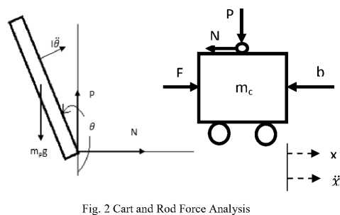
The structure of the inverted pendulum is as shown in the Fig. 1. After ignoring the air resistance and other frictions, 1-stage linear IP can be simplified as a system of cart and rod, as shown in Fig. 2.

Let’s define [3]

M: Cart Mass = 1.096 Kg

m: Rod Mass = 0.1096 Kg

b: Friction Coefficient of the Cart = 0.1 N/m/sec

I: Rod Inertia = 0.0034 Kg*m*m

l: Distance from the rod axis rotation center to the rod mass center=0.25m

F: Force acting on the cart

x: Cart position

ф: Angle between the rod and the vertical direction

ϴ : Angle between the rod and the vertically downward direction

From the forces in the horizontal direction, we obtain:

̈=  -  ̇-                 (1)

(  +  ) ̈+  ̇+    ̈     -    ̇      =  (2)

The equilibrium state is taken as;

X =[x ẋ θ  θ]̇ =[ 0 0 0 0]

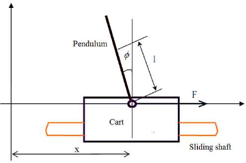
Fig. 1 Inverted Pendulum System Model

Analyze the force in the vertical direction, and then we have

• -    =      ()

• -    =-   ̈    -

• Combining two, we get the second dynamic equation:

( +    ) ̈+          =-   ̈(3)

The two dynamic equations are:

(  +  ) ̈+  ̇+    ̈     -    ̇      =(4)

( +    ) ̈+          =-   ̈(5)

( +   )ф()  -   ф()=   ()(6)

(  +  ) ()  +  () -  ф()  =  () (7)

The output angle is φ, solving the first equation:

()=

( +    )

s2

The state space equation can then be written as:

[ΦΦxх̈̇̈]=⎢⎢⎢

()

()

-mlb

()

m2gl2

()

()

()

x ẋ Φ

• Φ̇

B. Mathematical Model of Inverted Pendulum

Fig. 2 is the force analysis of cart and rod system. N and P denote the interactive force of cart and rod in the horizontal and vertical direction respectively.

+

(        )

(       )

ml

⎣ (       )          ⎦

y-M 010][i]+[0b   «

• III.    Reinforcement Learning

The reinforcement learning does not specify as to how to solve a particular problem [4], instead the final goal is defined in terms of the terminal states and based on that the state-action value function is to be approximated based on rewards or punishments (negative rewards) given by the environment on the goodness of the selected action in the next observed state. So it focuses on what should be done and not that how it should be done.

In reinforcement learning, there is no external supervisor to critically judge the control action chosen at each time step rather the learning system is told indirectly by the agent about the effect of its chosen control action in a way that it describes the quality of the action chosen. The study of reinforcement learning relates to credit assignment, where, given the performance (results) of a process, one has to distribute reward or blame to the individual elements contributing to that performance [5]. This idea may further become complicated if there is a large number of actions, which are collectively awarded a delayed reinforcement. The nonlinear behavior of many practical systems and the unavailability of quantitative data regarding the inputoutput relations make the analytical modeling of these systems very difficult [6]. Fig. 3 shows the agentenvironment interaction block diagram

States

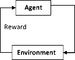
Fig. 3 The Reinforcement learning framework

Action

Most of RL algorithms are based on approximating value functions of state-action pairs that estimate how good or how bad it is for the agent to perform a chosen action in a given state. One of the very well-known methods of RL is Q-learning [6], which tries to estimate the floating point solution of the Bellman's equation given as in (13). But it is difficult to deal with continuous states environment and actions, using ordinary Q-learning because it can only deal with discrete states and actions. So to avoid these problems, we need to combine this Q-learning method with other generalization methods which can work in the continuous time environment. Some other authors too have extended the Q-learning method to handle the continuous time situation with continuous state spaces by using function approximation [8]. In these works, neural networks are used to approximate the value function pertaining to specific situations [9]. But these works still works on discrete actions and cannot handle continuous-valued actions.

• A.    Markovian Decision Problems

Markov decision processes (MDPs) have been widely used to model controlled dynamical systems in control theory. Let S = {1 . . . n} denote the discrete set of states of the system, and let A = {a1 , .... , am) be the discrete set of actions available to the system. The probability of making a transition from state x to state x' on action u is denoted by Pxx'(u) and the reward obtained from this transition is denoted by r(x,u). A policy maps each state to a probability distribution over actions. For any policy π, we define a value function:

^(%) - E^ о У ^t₊ 1 1х о -х}      (10)

which is the expected value of the infinite-horizon sum of the discounted rewards when the system starts in state x and the policy π is followed forever. Note that r_t and x_t , are the reward and state respectively at time-step t , and ( r t , x t ) is a stochastic process, where ( r t+1 ,x t+1 ) depends only on ( x t , u t ). The discount factor, 0 ≤ γ ≤ 1 , makes future rewards less valuable than more immediate rewards.

The solution of an MDP is an optimal policy π* that simultaneously maximizes the value of every state x ∈ S . The value function associated with π* is denoted by V *. It is often convenient to associate values not with states but with state-action pairs whenever there is no explicit model of the system. These values called Q-values in Q-learning [10] are defined as follows

Q^{л (}х,и) - ^Р _xxf⁽и)(г⁽х,и) + уУ^л(х'))    (11)

Q *(х,и) - ^Р_ххЧи)(г(х,и) + уГ(% ' )) (12)

where x' is the random next state on executing action u in state x .

The Bellman's equation is given by:

и

Jk ⁽О ^- ^ ^^x aeA(i) ^P i₇' ⁽u⁾[^[.g⁽ ij',u^)]+ .„

7 = 1

[ у/ к - 1С/Э ]}              (13)

Many optimizing algorithms as well as reinforcement learning algorithms try to find the solution of this Bellman's equation.

• B.    Q-Learning

To compute the policy which maps the states to actions, the Q-learning algorithm is been employed. Q-learning algorithm gives the fixed point solution of the Bellmen's optimality equation through iterations. One of the most important breakthroughs in reinforcement learning was the development of an off-policy TD control algorithm known as Q-learning [4]. Its simplest form, 1-step Q-learning is defined by.

Q ( st , a_t )← Q ( st , a_t ) + ∝ [ r_t+i + …

Y ∗ max_aQ ( ^st+l , ^at+l )- Q ( ^st , a_t )]  (14)

where, α is the step size parameter, also known as the learning rate, γ is the discount factor, s t is the previous state, s t+1 is the new observed state and the a t+1 is the action taken in that state, r t+1 , is the reward in this state. Q(s,a) hence gives a value which tells gives the desirability of choosing that action a when in the state s . The Q-learning algorithm is implemented as follows [4]:

Initialize Q(s,a) arbitrarily

Repeat (for each episode):

Initialize s

Repeat (for each step of episode):

Choose a from s using policy derived from Q

(e.g. ϵ-greedy[4])

Take action a, observe r, s'

Q(s, a) ←Ԛ(ѕ, а)+ ∝ [rt+1 +γ maxa'Q(ѕ ,а)-Ԛ(ѕ, а)] s ← s'

until s is terminal.

S is the set of discrete states and A is the set of discrete actions. After each iteration, the action is chosen either greedily or randomly and is applied to the system and the next state is observed, then the reward is calculated and based on that, the Q-value is updated. The agent environment interaction is as shown in the fig. 3. After number of trials the actions which give satisfactory performance can be identified and the policy which gives maximum award can be identified by moving along the action with max Q-value in the Q-table. In this way the system is formed and results are obtained and are shown in the result section.

• IV.    Fuzzy Control

Fuzzy logic systems are expressed in linguistic terms to make its rule very close to our natural language. So fuzzy logic controller is a type of expert system which is based on if–then type of rules, in which premises and conclusions are represented with the help of linguistic terms or linguistic variable. Same nature of these rules as our natural language makes these fuzzy systems very easily readable and allows us a very easy introduction of a priori knowledge in the rule base of the system. While classical control methods need analytical modeling of tasks, these fuzzy logic controllers are usually designed by incorporating the knowledge of the experts in the rule base. But, this incorporation of experts’ a priori knowledge is not always easy or possible to realize, especially for the conclusions of the rules in the conclusion parts. In fact, problems can arise due to disagreements between experts, from decision rules that are difficult to structure or incorporate, or due to a large number of variables that are necessary to solve the control problem at hand.

• V.    Tuning of Fuzzy Controller Using Temporal Difference Based Q-Learning

The proposed tuning method of the fuzzy logic controller is a modified version of the actor-critic architecture as shown in the fig. 4.

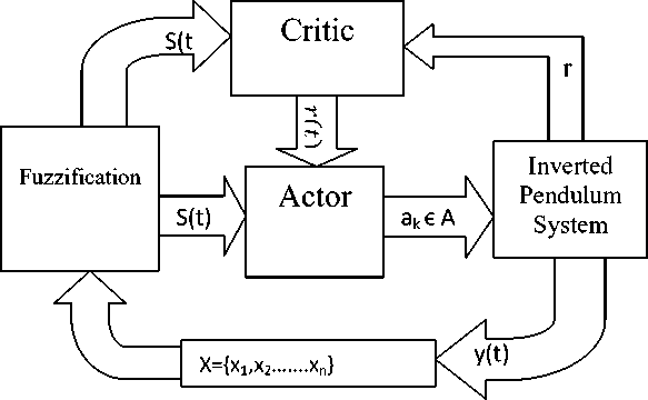
Fig. 4 Actor-Critic Architecture

The aim of this paper is to introduce a tuning method for Takagi-Sugeno type of fuzzy logic controller. In this paper the consequence part of the fuzzy logic controller is tuned through temporal difference based Q-learning. The rule base is a linguistic description of the controller, which yields a consequence in terms of what should be the action after each rule. Then the weighted sum of all the action produced by all the rules is computed. The task is to find the suitable action for every rule.

Unlike the ordinary fuzzy logic controller, here we considered many possible consequences or discrete actions A= {a1 , .... , an) attached to single rule and hence all the rules have many actions to chose from. Each rule contains a Q-value associated with it. The rules are written as follows:

Ri : If x is Xi then u1 is a1 with Q(Xi , a1)

or a2 with Q(Xi , a2)

or an with Q(X i , a n )

The continuous action performed by the agent for a particular state is calculated by the weighted sum of the actions concluded in the fired rules that describe this state and are determined by the Q-values of the actions which in turn is to be calculated so that yields a maximum discounted future rewards. The weights are the normalized firing strengths vector of the rules. The TD method is used to update the Q-values of the elected actions according to their contributions and the reinforcement signal obtained from the environment. The reward is calculated using the reward function, which yields a numerical value after each global action, is performed on the environment. When we observe the next state, if the discount factor is γ, then the discounted future reward may be calculated as given in (15).

Rd= Y∗ maxaQ (st+l, G-t+l)-Q($t, at)(15)

If the reward is rt+1 in the next observed state and the learning rate is α then the total change in the Q-value can be calculated as given in (16).

Rl= ∝ [rt+1 + γ mаx a'Ԛ(ѕ ,а ) - Ԛ(ѕ, а)](16)

Hence, the Q-value can be updated for the each rule as given in (17).

Q ( ^st , a_t )← Q ( ^st , a._t ) + ∝ [ r_t+i + …

• Y∗ maxaQ(st+l, at+l)-Q(st , at)](17)

Equation (15) represents the learning component from the future rewards. This component is used to extract a better policy from the rewards instead of following the best rewards. Because at the time of learning the state which leads to the terminal state or in some more favorable state may have less rewards then other states in that situation. So the future states that we might come across must have a component in the present state-action value calculation. The discounted reward is calculated using temporal difference. Initially all the Q-values are initialized to zero.

During initial runs the performance of the system is poor, because of the exploring actions of the RL, because it has to explore all the actions for the future.

But as the number of runs increases, the exploring is reduced and the exploiting of explored actions increases. Hence the performance of the system improves gradually as the number of action explored, increases. In the result section, a failed trajectory is shown during the initial run at the time of exploring, then the stable trajectory are also shown in Fig. 6. Initially the probability of random action selection is kept high to explore most of the actions of the system and then it gradually lowered to improve the performance of the system and exploiting those actions which gives highest rewards.

This tuning algorithm is checked on 25 rules corresponding to two input variable having five membership functions each. Each rule has ten discrete actions from which it has to select one action which gives maximum reinforcement (positive reinforcement) and in turn maximizes the total reward received in the long run. The learning task is to select local action such that when global action computed using the weighted sum of the firing strength of the rules gives the maximum reward in the long run and hence able to keep the pole in the upright position.

• VI. Result

  To stabilize the pendulum the fuzzy rules are written for control of angle and the change in angle having five triangular membership function each, hence making a total of 25 rules. Considering only angle does not mean we are not considering the position of the cart. The position of the cart is controlled in a way that the agent is punished whenever the cart touches either side of the track. The reward function has to be designed such that it gives maximum reward when the pole is near to its equilibrium point and punishes when goes far from equilibrium point. We assumed that the system is stable as long as its angle remains in the limit of -12 degree to +12 degree and the cart's position does not go beyond the -2.4 m to + 2.4 m. So a failure occurs when |θ| > 12º or |x| > 2.4 m. The success is when the pole stays within both these ranges for at least 5000 time steps.

The parameters taken for the system for the learning algorithm are given in table I.

Table 1 Parametres used for RL algorithm

Symbol	Name	Value
Α	Learning rate	0.3
Γ	Discount factor	1.0
Τ	Time constant	0.005

The simulated system runs in the episodes. A single episode means a single cart-pole run till the failure or till 5000 time steps. Time steps indicate the total time while the pole remains in the vertical upright position without a failure. Fig. 5 represents a failed trajectory in the starting of the cart-pole simulation run. That means in the starting episode when the system has not learned sufficiently. The trajectory shows a diversion of the pole angle from the equilibrium point as the time increases due to the random actions selection.

Fig. 5 shows the trajectory of the pendulum when the learning is in starting phase. It is clear from the graph that the pole is going to be unstable and the trajectory is diverting away from the equilibrium point because in starting the exploring of the action must be done in order to know the quality of different actions. So initially the probability of random action selection over the greedy action selection is high, hence results in an exploring mechanism which later is reduced as the exploring increases. One must better take care of exploration Vs exploitation trade-off. As exploring leads to system failure because of taking random actions and exploiting prevents us to know actions which are not yet been explored, hence might prevent from taking some best actions.

Fig. 6 shows the trajectory after sufficient number of episode executed and the system has explored sufficient so that it is able remain in the limit of |θ| > 12º and a trajectory converging to the equilibrium point is shown.

Fig. 7 and fig. 8 shows the graph of the number of steps taken in the particular episode. It is clear from the graph that initially, the system fails many times because it does not know what good actions are. But then after exploration, it is finally able to stand in the vertical upright position. The learning time to control the pendulum in the upright position may vary for different time of running due its random action selection nature. The two cases are shown in the fig. 7 and fig. 8. One is learned in the 45th episode while in another case it has to wait until the 271st episode.

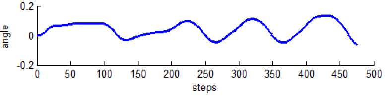
Fig. 5 Unstable Trajectory of angle Vs steps

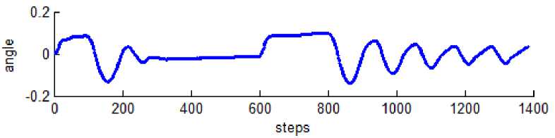
Fig. 6 Stable trajectory of angle Vs steps

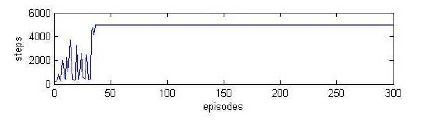
Fig. 7 Number of steps Vs Episode

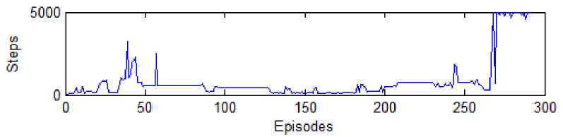
Fig. 8 Number of steps Vs Episode