Temporal Weather Prediction using Back Propagation based Genetic Algorithm Technique

Published Online November 2014 in MECS                                Modern Education x                           i          v                                                 ■ ancj computer Science

To be able to predict the future has been a dream of mankind since it became aware of its environment and its ability to manipulate it. Prediction is a phenomenon of knowing what may happen to a system in the next coming time periods. Weather is a time series based continuous, data-intensive, and dynamic process. Neural networks are suitable for solving non-linear problems that are difficult to be solved by the traditional techniques. Most meteorological processes often exhibit temporal and spatial variability, and are further plagued by issues of nonlinearity of physical processes, conflicting spatial and temporal scale and uncertainty in parameter estimates [7]. The artificial neural networks exhibit capability to extract the relationship between the inputs and outputs of a process, without the physics being explicitly provided. Thus, neural networks are well suited to forecast weather.

This article introduces a temporal weather prediction model that utilizes the strengths of two powerful artificial intelligent techniques: Back propagation algorithm and genetic algorithms taking time series based prediction into consideration.

• A.    Temporal Weather Prediction

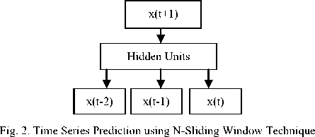
Temporal forecasting or time series prediction means prediction of future data values by taking existing or past data series as reference. Formally saying, time series prediction takes an existing series of data x(t-n),.., x(t-2), x(t-1), x(t) and forecasts the data values x(t+1), x(t+2),…, x(t+m) [9].

• B.    Back Propagation Algorithm

Back propagation using gradient descent technique suffers from the scaling problem. It works well on simple training problems. However, as the problem complexity increases, the performance of back propagation falls off rapidly because of the fact that gradient search techniques tend to get trapped at local minima, thus making for very slow training [15]. If the number of hidden neurons is increased, the number of independent variable of the error function also increases and the computing time also increases rapidly [5]. Several attempts have been made by various researchers to solve these problems using genetic algorithms.

• C.    Genetic Algorithms

Genetic algorithm is similar to the natural evolution process where a population of a specific species adapts to the natural environment under consideration, a population of designs is created and then allowed to evolve in order to adapt to the design environment under consideration for solving optimization problems [1].

As compared with back propagation, genetic algorithm is more qualified for neural networks as it is good at global searching (not in one direction) and it works with a population of points instead of a single point. Secondly, genetic algorithms work with a string coding of variables instead of the variables which requires only function values at discrete points, a discrete function can be handled with no extra cost [10].

Also inherently parallel nature of genetic algorithms makes the processing faster as compared to the back propagation algorithm. Another merit of genetic algorithm is that it is easy to be implemented by hardware. First of all, the required precision is not high. Second, if binary encoding is adopted, the results can be directly reflected to digital storage. The last, the arithmetic operation is simple, which is quite favorable for hardware implementation [14]. These benefits of genetic algorithms encourage researchers to combine both the artificial intelligent techniques together to generate hybrid models.

• D.    Hybrid Techniques

In order to solve the problems of back propagation algorithm, efforts have been made to integrate it with the genetic algorithms [12]. In the field of weather forecasting, the research has been done for the hybridization of back propagation with the genetic algorithms using the above mentioned technique. The latest weather forecasting model lays stress on the hybridization of back propagation and genetic algorithm for training the neural networks to predict weather parameters assuming that they are independent of each other and their temporal relation with one another is not considered. All these limitations sowed the seeds for the present research.

The remainder of the article is organized as follows: materials and methods used are detailed in Section II, training and testing methods are given in Section III, performance of the proposed technique is shown through results in section IV, and finally the conclusions are summarized in Section V.

• II.    Materials And Methods

The proposed work involves training a back propagation network through genetic algorithms so as to blend the merits of both the techniques in weather forecasting by discarding the assumption that weather parameters are independent of each other, having no temporal relation between them and no time series trend present in the weather data. Also it will try to solve the problems incurred in the hybrid BP/GA technique and provide a complete and accurate time series weather prediction model as shown in Fig. 1.

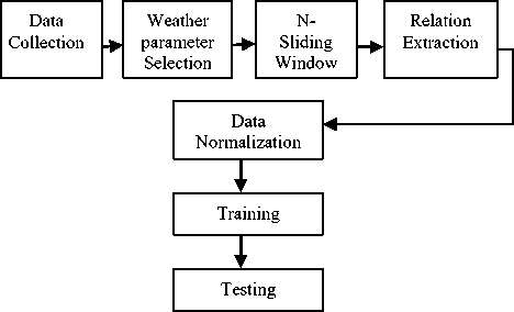
Fig. 1. Steps to design Time Series Weather Prediction Model

• A.    Collection of Data

First step in the design of rainfall prediction model is to collect data obtained through instruments. The data used in this research are the daily rainfall data. The data in the un-normalized form have been collected from Punjab Agriculture University, Ludhiana for the Ludhiana city of Punjab.

• B.    Selection of Weather Parameters

Daily weather parameters collected from the “Meteorological Department of Punjab Agriculture University, Ludhiana (Punjab)” are shown in table 1

along with their units of measurement. The parameters chosen in this setup for the prediction are mean air temperature (ºC), relative humidity (%) and daily rainfall (mm).

Table 1. Weather Parameters

Sr. No.	Meteorological Variables	Unit
1	Mean Air Temperature	ºC
2	Rainfall	Mm
3	Relative Humidity	%

• C.    N-Sliding Window

Work in neural networks has concentrated on forecasting future developments of the time series from values of x up to the current time. Formally, this can be stated as: find a function f(x): N→R such as to obtain an estimate of x at time t + d, from the N time steps back from time t, so that:

x ( t + d ) = f ( x ( t ), x ( t - 1 ), ..., x ( t - N + 1 ))          (1)

x (t + d ) = f(y (t))

where y(t) is the N-ary vector of lagged values.

The standard neural network method of performing time series prediction is to induce the function ƒ using any feed-forward function approximating neural network architecture, using a set of N-tuples as inputs and a single output as the target value of the network [2]. Fig. 1 gives the basic architecture.

This method is often called sliding window technique as the N-tuple input slides over the full training set which is mathematically known as the moving average and is calculated progressively as an average of N number data values over a certain period [13]. For a data set, represented by d_t, d_t-1, d_t-2 ,………………., d₀, where d_t is present and d 0 is the first data value, the moving average with a sliding window of period N is given as

MA n =

d t + d t-1 + d t-2 +………..+ d 0

N

• D.    Relation Extraction

In certain cases, the weather parameter to be forecast can be estimated based on the features, obtained from the past data of same parameter. However, in some cases the parameter to be forecast exhibits a strong dependence on other weather parameters also. In such cases the input to the network should include the features extracted from other weather parameters also. Therefore, to forecast each parameter, input variables are decided in such a manner that those features are included in the form of trends established by them over a definite period [8]. As some information is needed to access whether a specific feature is suitable for the model or not for inclusion in input data set, the selection of the features is made by correlating these features with the parameter to be estimated. The statistical indicators, which can be used as input features for the model, are as follows.

• (a)    Day Number: It is fed to the network as first input to keep track of the day for which the network is to be trained.

• (b)    Moving Average: It is calculated progressively as an average of N number data values over the certain period.

• (c)    Oscillator (OSC): Oscillator is used to indicate the rising or trailing trend present in the time series. It is defined as difference of moving averages or exponential moving averages of two different periods:

OSC = MAn1-MAn2

where N1 and N2 are different periods and N1>N2.

These features will act as input to the network along with the dependent parameter moving averages as shown in table 2.

Table 2. Features for Estimating Weather Parameters

Parameter	Inputs	Output
Features of mean air temperature	Day No Moving Average Oscillator	Mean Air Temperature
Features of dependent parameters	Moving Average (rainfall) Moving Average (humidity)
Features of daily rainfall	Day No Moving Average Oscillator	Daily Rainfall
Features of dependent parameters	Moving Average (temperature) Moving Average (humidity)
Features of relative humidity	Day No Moving Average Oscillator	Relative Humidity
Features of dependent parameters	Moving Average (temperature) Moving Average (rainfall)

• E.    Data Normalization

After the collection of data and selection of the weather parameters, next issue is the normalization of data. Neural networks generally provide improved performance with normalized data. The use of original data to network may cause convergence problem [6]. All the weather data sets were, therefore, transformed into values between 0 and 1 by dividing the difference of actual value d_t and minimum value d_min by the difference of maximum value d max and minimum value to obtain the normalized data d norm as in (5).

ddt-dmin norm=                                          (5)

d max -d min

The main goal of normalization, in combination with weight initialization, is to allow the squashed activity function to work at least at the beginning of the learning phase. Thus, the gradient, which is a function of the derivative of the nonlinearity, will always be different from zero. At the end of the algorithm, the outputs are denormalized into the original data format for achieving the desired result.

• III.    Methodology: Training and Testing

The network is trained using the hybrid back propagation based genetic algorithm technique as in Fig. 3.

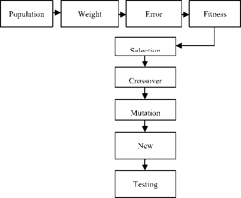
Fig. 3. The block diagram of training procedure

• A.    Population Generation

At this step, two main issues need to be solved namely the determination of population size and the initialization of population. As chromosomes form the initial population so population size must be specified. This parameter determines how many chromosomes should be present in the population at any one time. The number of chromosomes present in the population depends on the length of a chromosome. Every chromosome consists of some number of genes. A particular number of weights are extracted from each chromosome depending upon the number of genes a chromosome have. This calculation is done as follows: Let the network configuration is l-m-n. Therefore, the numbers of weights (genes) to be determined are as in (6).

W = ( l + n ) x m (6)

With each gene being a real number, and taking the gene length as d, the string representing the chromosomes of weights will have a length of C , as in (7).

C = W x d (7)

It represents the weight matrices of the input-hidden-output layers. Two main methods are followed for initializing the population. One is to randomly generate the population. This method is followed when we are not particularly taking the initial population as set of alternative solutions. Another method is generating the population with some known good solutions and is followed when domain of solutions is fixed like in case of Travelling Salesman Problem, each gene denotes the city and chromosome denotes the tour plan. The present research uses random initialization method as it aims at obtaining the optimal set of weights for forecasting the outputs.

• B.    Weight Extraction

Before hybrid technique can be put to work on any problem, a method is needed to encode potential solutions to that problem in a form that computer can process. One common approach is to encode solutions as binary string (0s and 1s) in which each string represents some aspect, real coding in which the particular value of an aspect is specified in real numbers, and string coding in which each letter stands for a particular aspect of the solution.

In the present work, real coding is used to encode the value of weights. As chromosomes are a set of genes and genes denote the weights, so real numbers will specify the weights of neurons. In the gradient based back propagation method, weights are taken as real numbers, similarly for the hybrid technique. Also the length of each gene is specified in the last section to be an integer d so that the weights extracted are with precision d-2 decimal places. The value of weights will be extracted from the randomly generated chromosomes keeping the following rule: If the most significant bit G5 of a gene G5G4G3G2G1 is a number less than or equal to d then the weight will be G4.G3G2G1 else the weight will be -G4.G3G2G1.

• C.    Error Calculation

After the extraction of weights, the product of inputs along with the weights is summed together and fed to the network for calculating the actual output. These outputs when compared with the desired output, error values are obtained. Root mean squared error is calculated instead of simply subtraction of actual output from desired output, in order to eliminate the negative values as in (8).

RMSE =

N

where DO is the desired output, FO is the forecasted output and N is the number of terms in data set.

• D.    Fitness Evaluation

The search for selecting an individual is guided by the fitness of each individual i.e. evaluating the quality of each chromosome. So, fitness function is evaluated by reciprocating the root mean squared error as in (9).

Fitness =

1 RMSE

where RMSE is the root mean squared error as given in (8). More the fitness value is, more the chances of a chromosome to be selected for reproducing an offspring are.

• E.    Selection (Elite Fitness Proportionate Selection

After the calculation of fitness of each individual in the population, individuals to act as parents are randomly selected. The selection method used in the present research is elite fitness proportionate with replacement. Fitness proportionate selection states that more fit individuals are more likely to be selected and partial elitism is there because the previous best fit individuals are also present in the new population so that they do not get lost and optimal solution is not lost in between the generations.

This method can further be used with replacement and without replacement. The selection process without replacement is not greedy as the best fit individuals are not replaced with the worst fit individuals. The best individual is not guaranteed to be selected and the worst individual will not necessarily be excluded. Individuals that are known to be inferior still have some chance of being selected. Second method is with replacement in which the worst fit individuals are replaced by best fit individuals. This is a greedy method but it is quite faster than the without replacement method.

• F.    Cross-over (Two-point Cross-over)

With the above criterion in mind, mating pool is prepared by replacing the individual with minimum fitness value by individual having maximum fitness value. The population is enriched with better individuals after reproduction phase is over.

Reproduction makes the clones of good strings in the mating pool but doesn’t create new strings. Cross-over operator is applied to mating pool with a hope that it would create a better string (offspring). The main aim of crossover is not only to search the parameter space but also the search is to be made in a way that information stored in the present string is maximally preserved as these parent strings are instances of good strings selected during the reproduction. The main crossover methods are single-site crossover in which search is not so extensive but information is preserved, two-point crossover in which search is extensive as well as information is preserved and uniform crossover in which search is extensive but information of parents is not preserved.

Some studies have shown, it is difficult to generalize the optimal crossover operator selection. So it is left to personal interest to select the crossover operator. In the present case to satisfy both the aims of crossover operator, two-point crossover method is chosen. Also if the newly created offspring is not so good, it will automatically be deleted in the next population. A crossover rate of 0.6 is used in the present research.

• G.    Mutation (Self-adaptive Variation)

Self adaptive variation/mutation is used which says the higher the fitness of individual is, the less the mutation probability is. In other words, the high fit off-springs will not be mutated and worst fit individuals will be mutated with a low probability. Mutation rate used in the present setup is 0.01.

• H.    Stopping Criteria

There must be some stopping criterion for the algorithm to get stopped. With the elite fitness proportionate selection with replacement, the network is considered to be trained when 95% of the individuals have same fitness value [11]. So, the algorithm gets stopped after the chromosomes achieve same value of fitness.

• I.    Testing

This procedure repeats itself till the network gets trained. After the training phase, testing is done with the set of weights obtained during the training phase. In the testing phase, the inputs are fed to the network along with the final weights and we obtain the outputs thereafter. The actual weather output is received only after the testing phase.

The major issues regarding neural network architecture is the selection of number of hidden neurons in the hidden layer. So a comparison for RMSE values has been done corresponding to different number of hidden neurons along with the population size and number of iterations in which the network can be sufficiently trained with minimum error value [4]. For each value of population, the program has been executed and the error has been calculated. Table III shows the variations in population size, number of neurons in hidden layer and the corresponding mean absolute percentage error values for the integrated BP/GA technique. Table 4 shows the features extracted from the data values of all the three weather parameters assuming them to be independent of each other.

Table 4. Extracted Features of Independent Weather Parameters

Weather Parameter	Day No.	MA	Oscillator	ROC	Moment
Temperature	26	19.8800	1.2000	-16.333	2.0000
	27	20.5000	-2.0000	-54.333	3.0000
	28	19.8000	1.0000	-16.000	4.0000
	29	20.3000	-1.9000	-55.493	5.0000
	30	21.8600	-2.5000	-49.523	6.0000
Rainfall	26	0.0001	0.0001	-1.6633	2.0000
	27	3.0000	3.0020	99.6433	4.0000
	28	1.6800	0.2031	99.9633	5.0000
	29	1.0200	0.1050	98.6532	6.0000
	30	0.4800	0.1031	99.7833	7.0000
Humidity	26	65.9800	-10.0011	-19.663	1.0000
	27	77.8800	6.1120	-20.663	2.0000
	28	72.6800	4.3460	-20.000	3.0000
	29	82.6800	8.3460	-24.663	4.0000
	30	67.6800	-5.4460	-12.963	5.0000

• IV.    Results and Discussion

The proposed model uses multilayer feed forward architecture that has one or more than one hidden layers. In this research, 5-3-1 neural network architecture has been used. The number of input neurons is 5 representing the extracted features, the number of hidden neurons is 3 for processing and the number of outputs is 1 representing the weather variable (amongst mean air temperature, relative humidity and rainfall) to be forecasted.

Table 3. Selection of Appropriate ANN Architecture

Network Architecture	Population Size	Hidden Neurons	No. of Iteration	RMSE Value
5-1-1	30	1	110*	1.10
5-2-1	60	2	140	0.86
5-3-1	90	3	220	0.42
5-4-1	120	4	282	1.47
5-5-1	150	5	425	1.85

Table 5. Extracted Features of Dependent Weather Parameters

Weather Parameter	Day No.	MA	Osc	depMA1	depMA2
Temperature	26	19.8800	1.2000	0.0001	65.9800
	27	20.5000	-2.0000	3.0000	77.8800
	28	19.8000	1.0000	1.6800	72.6800
	29	20.3000	-1.9000	1.0200	82.6800
	30	21.8600	-2.5000	0.4800	67.6800
Rainfall	26	0.0001	0.0001	19.8800	65.9800
	27	3.0000	3.0020	20.5000	77.8800
	28	1.6800	0.2031	19.8000	72.6800
	29	1.0200	0.1050	20.3000	82.6800
	30	0.4800	0.1031	21.8600	67.6800
Humidity	26	65.9800	-10.001	19.8800	0.0001
	27	77.8800	6.1120	20.5000	3.0000
	28	72.6800	4.3460	19.8000	1.6800
	29	82.6800	8.3460	20.3000	1.0200
	30	67.6800	-5.4460	21.8600	0.4800

Table 5 shows the extracted features of dependent weather parameters for all the three weather parameters: mean air temperature, daily rainfall and relative humidity.

After feeding the inputs, forecasted output for independent as well as dependent parameters are obtained. The error values corresponding to weather parameters: mean air temperature, daily rainfall and relative humidity are shown in table 6 along with the desired output and the forecasted output for the proposed model.

trapped into local minima and hence gives inaccurate output values. So, the comparison shows clearly that the hybrid model is more suitable to predict weather than the traditional gradient based back propagation algorithm because in all the cases- mean air temperature, daily rainfall and relative humidity; the hybrid BP/GA techniques are more close to the desired output than the back propagation algorithm.

Table 6. Prediction of Weather Parameters

Weather Parameter	Day No.	DO	Independent Weather Parameters		Dependent Weather Parameters
			FO	Error Value	FO	Error Value
Temperature (ºC)	1	21.8	24.2	2.4	23.5	1.7
	2	22.5	23.6	1.1	22.9	0.4
	3	19.8	18.2	1.6	19.4	0.4
	4	18.9	18.2	0.7	18.5	0.4
	5	22.0	19.7	2.3	22.4	0.4
Rainfall (mm)	1	0.0	0.0	0	0.3	0.3
	2	4.5	0.6	3.9	5.9	1.4
	3	0.4	0.0	0.4	0.0	0.4
	4	1.0	0.0	1.0	0.7	0.3
	5	0.0	0.8	0.8	0.0	0
Humidity (%)	1	65	57.3	7.7	64.8	0.2
	2	67	68.5	1.5	71.3	4.3
	3	62	62.8	0.8	71.6	9.6
	4	72	70.6	1.4	71.6	0.4
	5	65	61.4	3.6	71.7	6.7

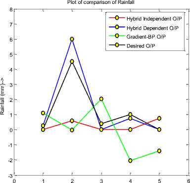
No. of days-->

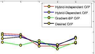
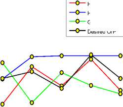
Fig. 5. Comparison of three techniques with desired output for rainfall

Fig. 4, 5 and 6 show the comparison of proposed technique with the previous ones.

Е

-5

-10

Plot of comparison of Temperature

Е

No. of days-->

Fig. 4. Comparison of three techniques with the desired output for temperature

This comparison is done to show which technique is more close to the desired output out of the three techniques. Negative values for daily rainfall parameter shows that the gradient based BP technique has get

Plot of comparison of Humidity

Hybrid-Independent O/P

Hybrid-Dependent O/P

Gradient-BP O/P

Desired O/P

No. of days-->

Fig. 6. Comparison of three techniques with desired output for humidity

Secondly, it is analysed that the time series based dependent weather prediction technique works well for the case of mean air temperature and daily rainfall but independent weather parameter technique is better than the dependent one for the case of relative humidity. In other words, the overall accuracy of the proposed time series weather prediction model based on back propagation algorithm with genetic algorithm technique is suitable to predict weather for all the three weather parameters than the gradient based back propagation technique and the independent weather parameter technique.

• V.    Conclusion

From the analysis above, it is easy to observe the compensability between back propagation algorithm (BP) and genetic algorithm (GA). The time series based hybrid technique can learn efficiently by combining the strengths of GA with BP. The proposed approach is more qualified for neural networks if only the requirement of a global searching is considered. It is good at global search (not in one direction) and it works with a population of points instead of a single point. Also it blends the merits of both deterministic gradient based algorithm BP and stochastic optimizing algorithm GA. By using local gradient information advantageously, the hybrid technique is more speed efficient than GA. Hence the use of time series based hybrid BP/GA technique is proposed for weather prediction.