The Feature Extraction to Determine the Wave’s Peaks in the Electrocardiogram Graphic Image

Published Online June 2017 in MECS DOI: 10.5815/ijigsp.2017.06.01

The electrocardiogram (henceforth ECG) is one of the useful assisting tools used to diagnose the heart abnormalities. Thus, ECG is usually used by the cardiologists to determine the abnormality of patients’ heart. ECG produces 12 lead recorded data on the special paper used to determine the patients’ heart abnormality, therefore the patients’ heart disorders is often determined according to the pattern from the ECG record (Fig. 1). The abnormality in the pattern of the 12 lead ECG record occurs when the heart beat is different from the normal sinus rhytm.

The 12 lead ECG record possesses some information representing the heart condition. The ECG pattern about the heart abnormalities is able to distinguish whether the heart is in normal or not. The determination of ECG peaks to get the main parameter needs special knowledge in the field of cardiology, thus it can prevent from the misinterpretation. In order to get the information from the ECG, a method to identify the ECG peaks is required. The common method used is pre-processing to improve the image quality obtained from the recorded data and feature extraction to determine the patterns of the ECG. The determination of the main parameters of the ECG recorded data will be useful to summarize the ECG result.

One of the ways used to help the feature extraction of heart abnormalities is by using the computer to determine the characteristic of the ECG pattern. The assisting tool to interpret the ECG result is very beneficial in the field [1]. The computer-assisted interpretation makes the determination of ECG pattern (P, QRS, and T), interval inter- peak, heart rate, and ST-deviation be carefully identified. This study aims at identifying the preprocessing method and the suitable feature extraction to determine the ECG peaks from the ECG recording result. In line with this aim, the researcher attempts to conduct a research to identify the ECG peaks (PQRST), heart rate, and ST-deviation based on the graphic image of the 12 lead ECG record.

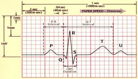
Fig.1. Electrocardiogram Wave

• II.    Related Work

The research about ECG has been done a lot, either in the form of image or signal. In [2], researched about the classification of ECG pattern by using fuzzy logic, preprocessing to identify the PR and RR peaks. In [3], the pre-processing to convert RGB (Red, Green, and Blue) to the grayscale by extraction of Prewitt edge detection, and ANN classification of propagation resilient) with accuracy 84.21%. Several stages pre-processing: binary, skew correction, salt-and-pepper filtering, and feature extraction by using Magnetic Resonance Spectrum (MNR) in [4]. The pre-processing is by altering RGB to grayscale and its extraction by selecting some methods, namely Wavelet Decomposition, Edge Detection, Gray Level Histogram, FFT, and Mean-Variance, the classification by using the ANN Feed-forward, the accuracy level of those five methods is Edge Detection (95.2%) in [5]. In [6], the pre-processing is by converting the RGB to grayscale by using the Welch method and the classification of ANN Backpropagation gets the accurate level 72.5%. The pre-processing use grayscale, dilation and clipped, as well as extraction to detect the R peak by the accurate result 95% [7]. The pre-processing by using the binary, reduction of noise and thinning, while the feature extraction by using the Transformation of Discreet Wavelet and PCA (Principal Component Analysis) [8]. The study of [9], the preprocessing is done by the image scanning with the whole accurate level 97.07%. In [10], the pre-processing by using the grayscale and binary, while the feature extraction changes the time scale and voltage. While [11], [12], [13], [14], [15], [16], and [17] conduct some researches about ECG signal.

The research done by [16], detects the R peak in ECG by using the Continuous Wavelet Transform (CWT). The signal data are taken from the Physiobank . The result shows the average reaches the level of 99.16%. In [16], suggests that it is developed to the wider area to extract other features (such as the P, Q, S, and T peaks), so that the information about ECG is more accurate.

This research is proposed to determine the ECG peaks (PQRST), the heart rate, and ST-deviation in the normal heart, ischemia, or arrhythmia, and use the 12 lead ECG record image data. The pre-processing is done through some steps, such as: segmentation (grayscale and binary), morphology (dilation and erosion), and the alteration to the ECG graphic image. The feature extraction is to find out the PQRST peaks, Heart Rate (HR), and ST-deviation. This study is expected to be able to improve the result of the ECG peak determination in some heart disturbances (ischemia and arrhythmia) or normal.

• III.    Methodology

The model developed in this study includes some steps, namely data preparation, pre-processing, and feature extraction as shown in Fig. 2. The ECG graphic image is taken from the scanning result of the ECG recorded data.

Pre-processing

Data Preparation

Feature Extraction

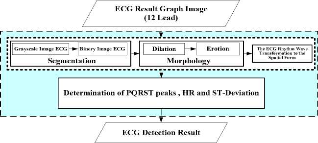
Fig.2. Determination Model Proposed ECG Peak

• A.    Data Preparation

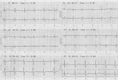
The data studied are the ECG graphic image in the form of the recorded data for three heart conditions (normal, arrhythmia, and ischemia). The ECG graphic image is taken from the scanning result of the 12 lead ECG record data in patients of Sardjito hospital of Yogyakarta in the heart polyclinic (Fig. 3). The study us limited to some things:

• 1.    The ECG data in this study are taken from the patients ≥ 18 years old,

• 2.    Not athlete ECG

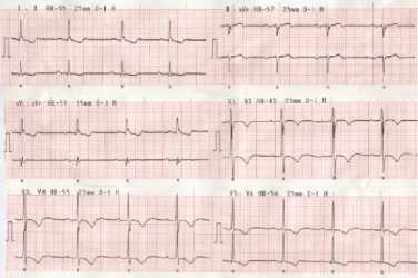
Fig.3. Example 12 lead ECG Image

The data preparation is done in some processes, namely data collection, ECG interpretation counseling, data scanning, and cropping is show in Fig. 4.

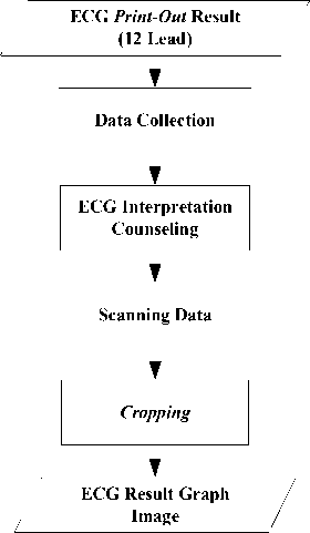
Fig.4. Data Preparation Process From ECG Print-out

Each result of the ECG recording is scanned, the result of the scanning is submitted. The scanning is done by using the resolution 600 dpi and the result is saved in the file with JPEG extension. The scanner resolution is 600 dpi , therefore the image element of one is taken [6].

600 point = 25.4 mm

1 point = 25.4 / 600 mm

1 point = 1 / 23.6 mm = 0.0423 mm

Thus obtained the conversion value to 1 pixel = 1 / 23.6 mm = 0.0423 mm. It means that if the image has the resolution of 600 dpi , then every 25.4 (1 inch) has 600 pixels.

The data submitted are validated by the cardiologists and they are classified into normal sinus rhythm, arrhythmia, and ischemia. The next step is to crop, the scanned the 12 lead ECG record is cropped. The cropping is done in each lead started from the beginning of the wave to the end (Fig. 5).

Cropping In

Lead V6

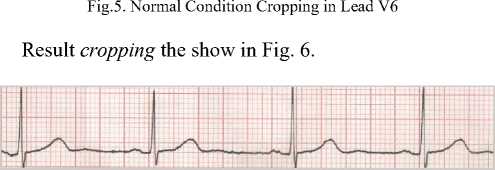
Fig.6. Cropping Normal Condition ECG in Lead V6

• B.    Pre-Processing

The next procedure is the pre-processing which is started by the segmentation process (grayscale and binary), morphology (dilation and erosion), and finally the transformation of the ECG rhythm wave image (Fig. 7).

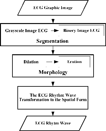
Fig.7. Pre-processing ECG Graphic Image

• a.    Segmentation

The image segmentation is a process of processing the image to separate the object region and the background region [18]. This segmentation uses two processes, namely the grayscale and binary. The segmentation process is done to remove the grid and convert it to the binary image (black and white), so the graphic is separated from the background. The binary image is a digital image which has only two possible colors, namely black and white. The formation of the binary image needs the grey limit which is used as the standard value. The pixel with bigger grey scale than the limit will be labeled as 1 and the pixel smaller than the limit will be labeled as 0. The method employed to determine the binary image in this study is the thresholding. When the thresholding is constant, the approach is called the global thresholding. One of the methods to choose the thresholding is by examining the image histogram visual. Another method in choosing the thresholding is the trial and error method, taking the different threshold up to one T value which gives good result according to the observer decision. This study uses the trial and error method. The threshold value used is 0.5, as from some trials, the value shows the good result (the graphic is able to be separated from the background well).

• b.    Morphology

The morphology is used so that the disconnected graphic will be connected again and the object size is good enough (similar to the original form). To improve the ECG graphic form, the morphology operation is done, namely dilation and erosion [19].

• c.    The ECG Rhythm Wave Transformation to the Spatial Form

The axis y from the ECG image becomes the ECG amplitude image and the axis x in the ECG reading becomes the time signal. If the image has 600 dpi resolution, every 25.4 mm (1 inch) has 600 pixels [34]. Therefore, the image width ( x ) in the mm is

X 25.4 mm and the height of the image is

X 25.4 mm . As the values in the ECG is amplitude time, the axis x (ECG width) is altered into the

Suppose the starting point ie (1,84) is shown in Fig. 8.

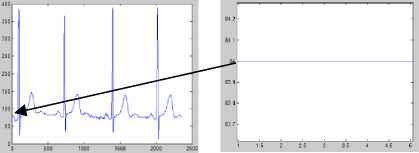
Fig.8. Start Point Illustration ECG

The calculation of a point (1,84) :

x’ = ^- x 25.4 x 0.04 600

x’ = ---x 25.4 x 0.04 600

x’ = 0.0017

whereas

y’ = -^У- x 25.4 x 0.1 600

y’ = -84 x 25.4 x 0.1 600

y’ = 0.3556

Thus the result of the calculation of (0.0017, 0.3556) is converted into the graphic (Fig. 9), namely:

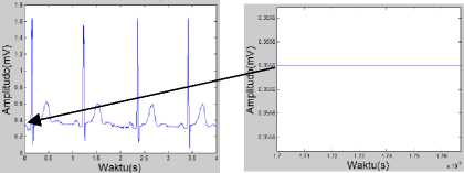
Fig.9. Illustration Calculation Results ECG

The whole scaling process result is showed in Fig. 10.

600 У

600 and

seconds. The recording rate used is 25 mm/second, in which 1 mm (one small square of the ECG paper) indicated 0.04 second, therefore for calculating the ECG period using equation (1) as follow:

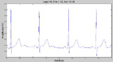
Fig.10. Scaling Process Results in ECG Normal Conditions Lead V6

x' = — X 25.4 x 0.04

Meanwhile, the axis y (the ECG height) is changed into mV in which in the ECG 1 mm (one small square of the ECG paper) shows 0.1 mV, so the ECG amplitude can be formulated by equation (2) as follows:

у' = — X 25.4 x 0.1

Ilustration:

Then, the amplitude value of ECG is normalized. The data normalization is done to place the input data in the certain range (between 0 to 1). It is to make the value of each data able to be calculated with its smaller value, so that the original data do not lose its characteristic. The normalization process aims to make the process become more effective by reducing the ECG image as far as the minimum value, so the normalized image minimum value is zero [6]. The normalization process uses the equation (3) [20]:

_N‘ ₌ V- N _min

^V max ^{- V}min

Which :

N’ = The data have been normalized.

N = The data will be normalized.

N max = The data maximum from the data set.

N min = The data minimum from the data set.

The result of this process will be used in the feature extraction process. Fig. 11 is the result of the normalization process.

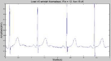
Fig.11. Normalized ECG Normal Condition in Lead V6

• C.    Feature Extraction

The feature extraction is a process of characteristic taking from an object in the image which will recognize or distinguish it from another object. The feature extraction uses the result of the pre-processing. In this study, the feature extraction will look for the ECG peaks (PQRST), heart rate, and ST-deviation. The determination of the QRS peaks uses the QRS algorithm [21].

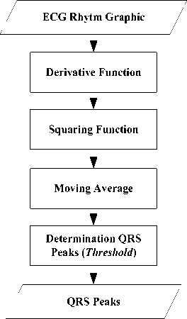
Fig.12. Process Algorithm Determining Pan-ompkins QRS wave (Pan and Tompkins, 1985)

The feature extraction begins with the process of derivative function, squaring, moving average, and the determination of the QRS peaks (Fig. 12).

• a.    Derivative Function

The first step is the derivative process, the standard technique to find out the high slope normally used to differentiate the QRS complex from another wave in ECG. The derivative process is carried out to limit the processed wave, in which only high ECG wave will pass, and muffle the low ECG wave. This limitation aims to find out the QRS signal structure and remove P and T signals. Thus, the derivative process presses the low wave component of P and T waves. In [22], suggest the derivative-based algorithm determine QRS. The derivative function developed to determine the QRS peaks is the derivative method of the first and second orders [22]. Further studied and evaluated by [23], [24], and [25]. The derivation function in this process combines the first and second derivative, in which x(n) is the input and y(n) is the output of the process.

The first order derivative with the absolute value approach as shows at equation (4).

УоОО = | x(n)-x(n-2)|         (4)

The second order derivative with the absolute value approaches in the three derivative spots as show at equation (5).

У1(п) = | y0(n) - y0(n - 2)|

У1(п) = |(x(n) - x(n - 2)) - (x(n - 2) - x(n - 4))| У1(п) = |x(n) - 2x(n - 2) + x(n - 4)|  (5)

Both results are calculated and combined [22], so the equation can be changed become equation (6):

У2(п) = 1.3 Уо(п) + 1.1 У1(п)         (6)

From the combination, the equation:

У2(п) = 1.3 Уо(п) + 1.1 У1(п)

У2(п) = 1.3(x(n) - x(n - 2)) + 1.1(x(n) - 2x(n - 2) + x(n - 4))

У2(п) = (1.3x(n) - 1.3x(n - 2)) + (1.1x(n) -2.2(x(n - 2)) + 1.1x(n - 4))

У(п) = 0.1 | - X(„—2) - 2X(„—1) + 2X(„+1) + X(„+2)|

The 0.1 value approaches the 1/8 value, so the equation can be simplified by (7) [21]:

У(п) = g | - x(n-2) - 2x(n-1) + 2x(n+1) + x(n+2)| in which :

y(n) : the output data from the derivative function, x(n) : the input data from the derivative function,

The input from this process is the normalized ECG rhythm graphic image data and the output is the ECG data of the derivative function (Fig. 13).

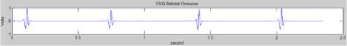
Fig.13. ECG After Derivative Function Process

• b.    Squaring Function

The result of the derivative function will be squared to get the absolute value from the ECG graphic. The squaring process aims to get the positive value. If the input of this process is y(n) and the output is p(n) , then to get the positive value uses the equation (8) [21]:

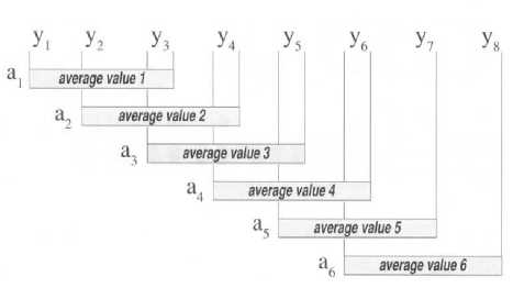
Fig.16. Ilustration Moving Everage Algorithm

P(n) = |y(n)|2                  (8)

The output of the square function to get the higher value is the characteristic of the R peak, while the peak of the valley will be positive. Fig. 15 shows the result of the squaring process. The input of the squaring function process is the output of the derivative function, and the output is the ECG absolute data.

Ilustration :

Example take first data derivative process result is 0.039772.

So,

p(n) = | y(n) |²

p( 1 ) = | 0.039772 |²

p( 1 ) = 0.0015818

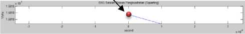
Fig.14. Ilustration Squaring Process Result

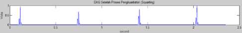
Fig.15. ECG After Squaring Process

• c.    Moving Average

The moving average is a simple mathematics technique to remove the data irregularity and shows the original data from a group of data. This technique is used to get the mean score of the close data and the result is approximately the original data. Every periodic wave can be considered as the group of data. The algorithm of moving average is done by taking two or more wave data, then the data are summed up and divided (by the total data), after that the first data from the wave is replaced by the average score, the step is repeated in the second, third, and so on up to the last data (Fig. 16). The final result is the second wave or derived from the moving average and which has the total data similar to the original wave [26].

The Fig. 16. displays how the moving average algorithm is applied to the data of a wave (represented by y ). From the illustration, the wave data which are respectively represented by “ y ” shows the moving average value. In this case, three data dots from the wave respectively are summed up, the total is divided by three, and it is plotted as the first data from the wave. This process is repeated in the second, third data, and so on up to the last one. The equation of the moving average can be calculated by (9) [26]:

ato^ Z n ^+(a-1) p(^)         (9)

Which:

a = the average value, n = position data point, s = the number of data is used, p = actual data point values,

Fig. 17. is the example of the comparison of moving average with on not moving average [26] .

Fig.17. Comparison of on not Moving Average (a) with Moving Average (11-point)(b)

In this case, the use of moving average is a process done to obtain data of ECG. As the illustration of the moving average in ECG, Fig. 18. can be used [27].

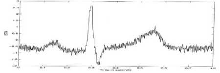
Fig.18. Ilustration Moving Average Process

From the Fig. 18, it is illustrated that moving average will be done by 8 (eight), so the result is the Fig. 19 [27].

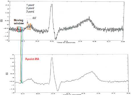
Fig.19. Illustration Process of Moving Average With 8 Point

Fig. 20 is the example of the comparison of the moving average from 8, 26, and 101 [27] .

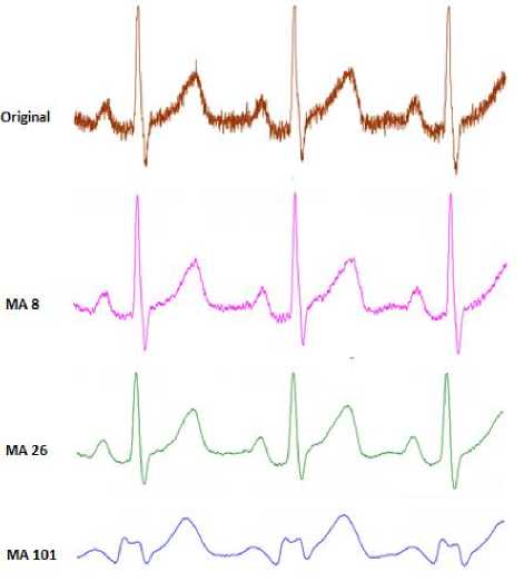
Fig.20. Comparison of Use Moving Average

In the case of ECG, the moving average process is aimed to obtain information about the characteristic of the wave due to the slope of the R wave [21]. This will create a suitable signal to the QRS of ECG. After the R parameter is found, the Q and S parameters can also be identified by marking the first and second valley in the QRS complex. The minimum dot which is located in between the left slope edge and the R peak is called Q. S is calculated by using the minimum dot in between the R peak and the right edge of ECG. The ups and downs of the edge are used to identify the time differences between the QRS complex.

Normally, S parameter (in the equation 10) is chosen experimentally. However, in some researches, the value of S ≈ 30s the appropriate value to determine QRS peaks [28]. The input from the moving average is the squaring function result. The result of the moving average process in lead V6 is displayed in Fig. 21. The input of this process is the ECG absolute data resulted from the squaring function and the output is the ECG peak data resulted from the moving average.

Fig.21. ECG After Moving Average Process

• d.    Determination of the R Peak

All ECG peaks contain P, R, and T peaks. Consequently, the selection has to be done to choose the R peak. There are some steps to select the R peak, namely the highest peak selection, threshold value determination, and R peak selection based on the threshold value [29]. Thresholding used to determine the QRS peaks in the high signal. The equation (10) is an equation used to identify the highest peak value:

Slope (и) > slope threshold         (10)

The last step in identifying the R peak is choosing the detected ECG peaks based on the threshold in equation (11) is:

threshold = q * max(z(n))        (11)

in which ƞ is the threshold parameter. If the local peak has the value above the threshold, so it is detected as the R peak (z(n)). If the local peak has the value below the threshold, so it is not the R peak. Fig. 22 shows the determination of the R peak. The algorithm used in determining the R peak is as follows:

• 1)    Examine all peaks and if there is a peak above the threshold limit, it means that it is the R peak.

• 2)    If the R peak has been found, the valley peak in the left side is detected as the Q peak and the valley peak in the right side is detected as the S peak.

• 3)    If there is a peak after the QRS peaks are found, examine the value if it is a half of the maximum value in the previous detection process. If yes, the peak is R peak. If not, it is T peak.

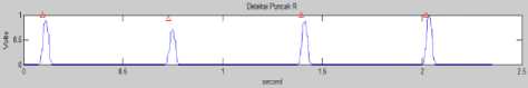
Fig.22. The Determination of Peak R ECG

• e.    Determination of the P Peak

P peak is the first peak in the heart cycle in ECG. The characteristic of the normal P wave is soft and not sharp, normal duration 0.08 - 0.10 second, not higher than 2.5 mm (0.25 mV). P peak precedes the QRS complex, which means one P peak has to be followed by one QRS complex. The threshold level is used as the reference to determine the location of P peak in the normal ECG. P-R normal interval from 120 – 200ms. P peak is also marked by the first positive peak in the left side of the R peak location [30].

• f.    Determination of the T Peak

The T peak determination is very significant to determine the ST-deviation. If the maximum steep in this wave is less than a half of the preceded QRS peak, it is detected as T peak. Otherwise, it is QRS peak [21]. The T peak determination by finding out the maximum value in the interval of R location in between 25 to 100. The T peak is less high than 5 mm, or the T peak is detected by the minimum T > 1/7 from the R or maximum < 2/3 from R. The T peak could be positive, negative, or biphasic. When the interval R-R is less than 360 ms (must be more than 200 ms), the determination is made to determine if the QRS peak has been found out correctly or it is the T peak.

• g.    Heart Rate

Heart rate is the number of one’s heart beat per period of time which is expressed in beats per minute (bpm). The heart rate us also called as R-R interval because it is normally measured the time interval in ECG wave. Calculating the heart rate can be done by determining the interval of R-R wave peak in equation (12). The interval between R-R marks the period of the heart beat which is converted to be heart rate [31]:

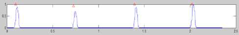
Fig.24. The determination of peak R-R In Process Heart Rate at Normal

Conditions Lead V6

As indicated in Fig. 24, the process of calculating the beats per minute is done by taking samples based on the R-R wave interval, then the interval based on the graphic as much as 0.75 – 0.09 = 0.66 second is derived (2.092 –

1.994

0.098 = 1.994, so the R-R interval average is      =

0.664). It means that the heart beats every interval 0.664 seconds (0.66 seconds). By the calculation of the beats 60

per minutes based on the formula used             , the value of    = 90.28 bpm is made.

Computation result:

R-R Interval =0.66 seconds/beat

Heart Rate=90.28 bpm h. ST-deviation

The ST-deviation is one of the ways to identify the heart defect. The ST-deviation is calculated from the S peak to T peak. The normal ST-Segment in the ST-deviation is in the isoelectric (Fig. 25).

HR =

In which :

R-R Interval

(bpm)

HR: Heart Rate

R-R Interval : the interval between R to R peaks in the ECG wave.

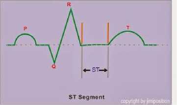
Fig.25. ST-Segment Normal Condition

The R-R interval is relatively constant from one beat to another (Fig. 23). The heart rate is calculated in the beats per minute (bpm). The value of the normal heart beat is between 60 to 100 [32]. If the heart beat is faster than the normal or slower, the arrhythmia occurs.

Some of the ST-Segment conditions are:

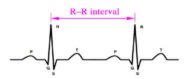
Fig.23. R to R Interval

• a.    Depression ST-Segment (the value is below the isoelectric line) > 1 mV (Fig. 26.a)

• b.    There are more than 1 ST-Segment depression (Fig. 26.b)

• c.    ST-Segment  depression can be horizontal,

downsloping or upsloping (Fig. 26.c)

Fig. 24 is the result of the R-R peak determination in the heart rate process .

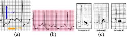
Fig.26. Some the ST-Segment Conditions

• a) Determination ST-deviation Algorithm

The algorithm used in determining the ST-deviation is as follows [33]:

Step 1: Read all peaks of ECG signals

Step 2: If any peak is 60% over the threshold, the peak is detected as R peak

Step 3: If minimum value (left of R peak) is in the interval of location R-50 to location R-10, the peak is detected as Q peak

Step 4: If minimum value (right of R peak) is in the interval of location R+5 to location R+10, the peak is detected as S peak

Step 5: If maximum value is in the interval of R+25 the peak is detected as R+100, the peak is detected as T peak

Step 6: ST-deviation count:

o PR= R_location – (S_Off – Q_Start)/2);

o ST = T_location – (T_Off – T_Start)/2);

o ST-deviation= abs(x(PR) - x(ST));

Step 7: Find X=| ST-deviation |.

X = ST-deviation value finally.

b)  ST-deviation Calculate

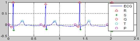
Fig.27. Calculate the ST-deviation for Normal Condition

Fig. 27 can be used as the reference to calculate the ST-deviation by using the mentioned calculation in the algorithm to determine the ST-deviation.

• a)    Find PR

PR = R_location – (S-Off – Q_Start)/2)

= 0.99661 – ((-0.0457 – (-0.0762))/2)

= 0.99661 – (0.0305 / 2)

= 0.99661 – (0.01525)

= 0.98136

• b)    Find ST

ST = T_location – (T_Off – T_Start)/2)

= 0.16942 – ((-0.0117 – (-0.0185))/2)

= 0.16942 – (0.0068 / 2)

= 0.16942 – 0.0034

= 0.16602

• c)    Find ST-Deviation

ST-Deviation = | PR – ST |

= | 0.98136 – 0.16602 |

= 0.81534

From the calculation, the ST-deviation value is 0.81 (0.81534).

• IV.    Result

The research finding is to detect the ECG peaks, the heart rate, and ST-deviation. From 266 the collected data, only 226 data are used after the counseling with the cardiologist. The result in this section is a description of methods in the methodology section presented consecutively. It started from pre-processing stage to feature extraction stage and ECG detection of PQRST peaks, heart rate, and ST-deviation.

• A.    Pre-Processing

ECG which had been collected and discussed with cardiologist was then scanned and cropped. The cropping result was then used as input of pre-processing. The output of pre-processing stage was the input of feature extraction stage. The pre-processing stage includes the segmentation process (grayscale and binary), morphology (dilation and erosion), and ECG graphic. The result of the sequence is presented in Table 1 using equation (1) to (4).

Table 1. Pre-Processing Normal Condition

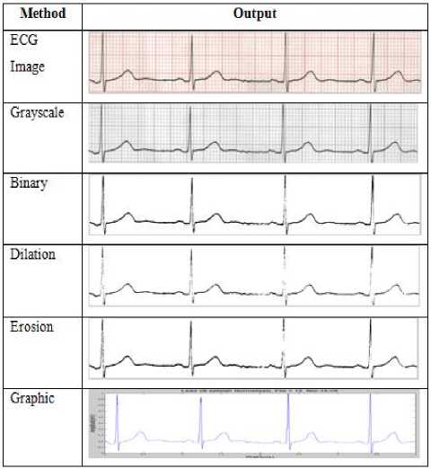
The final process in the pre-processing is in the form of ECG image which is transformed into the graphic.

• B.    Feature Extraction

After the pre-processing, the next step is the feature extraction. Feature extraction stage was the second stage and had very important role in determining the peaks of EKG waves. The input in the feature extraction is the image of the ECG rhythm graphic spatial interpretation. The feature extraction identifies the ECG peaks (PQRST), the heart rate, and ST-deviation. Based on the equation (5) to (13), the result is taken as displayed in Fig. 28, Fig. 29, and Fig. 30.

a. ECG Determination in Normal Condition

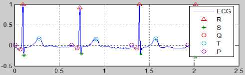
Fig.28. Result of the ECG Determination Process to Normal Condition

Fig. 28 is the result of EKG feature extraction in normal condition. The value of each peak PQRST, HR and ST-deviation in Fig. 28 as below:

High	Wave	P	=	0.00997 mV
High	Wave	P	=	0.00922 mV
High	Wave	P	=	0.01000 mV
High	Wave	P	=	0.01000 mV
High	Wave	Q	=	-0.09997 mV
High	Wave	Q	=	-0.06263 mV
High	Wave	Q	=	-0.08639 mV
High	Wave	Q	=	-0.08639 mV
High	Wave	R	=	0.99661 mV
High	Wave	R	=	0.92192 mV
High	Wave	R	=	1.00000 mV
High	Wave	R	=	1.00000 mV
High	Wave	S	=	-0.23916 mV
High	Wave	S	=	-0.19842 mV
High	Wave	S	=	-0.20861 mV
High	Wave	S	=	-0.27990 mV
High	Wave	T	=	0.16942 mV
High	Wave	T	=	0.15673 mV
High	Wave	T	=	0.17000 mV
High	Wave	T	=	0.17000 mV
R-R I	interval		=	0.66 seconds/beat
Heart	. Rate		=	90.28 bpm
ST-Deviation			=	0.81534

High	Wave	P	= 0	.00498	mV
High	Wave	P	= 0	.00461	nV
High	Wave	P	= 0	.00825	mV
High	Wave	P	= 0	.01079	mV
High	Wave	P	= 0	.00643	mV
High	Wave	Q	= -	0.22011	mV
High	Wave	Q	= -	0.24917	mV
High	Wave	Q	= -	0.24191	mV
High	Wave	Q	= -	0.15473	mV
High	Wave	Q	= -	0.20558	mV
High	Wave	R	= 0	.04977	mV
High	Wave	R	= 0	.04614	mV
High	Wave	R	= 0	.08246	mV
High	Wave	R	= 0	.10789	mV
High	Wave	R	= 0	.06430	mV
High	Wave	S	= -	2.28329	mV
High	Wave	S	= -	2.28329	mV
High	Wave	s	= -	2.30000	mV
High	Wave	s	= -	2.23316	mV
High	Wave	s	= -	2.23316	mV
High	Wave	T	= 0	.90432	mV
High	Wave	T	= 0	.85455	mV
High	Wave	T	= 0	.85455	mV
High	Wave	T	= 0	.93916	mV
High	Wave	T	= 0	.95613	mV

R-R Interval     = 0.81 seconds/beat

Heart Rate        = 74.04 bpm

ST-Deviation     = 1.75600

c. ECG Determination With Heart Rate > 100

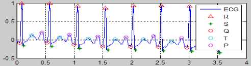
Fig.30. Result of the ECG Determination Process with Hear Rate > 100

b. ECG Determination With ST-deviation > 1

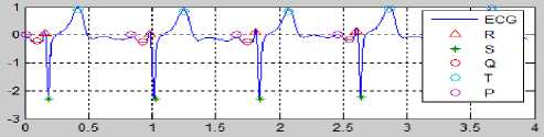
Fig.29. Result of the ECG Determination Process with ST-deviation >1

Fig. 30 is the result of EKG with heart rate > 100. Heart rate was determined by equation (13). The value of each peak PQRST, HR and ST-deviation in Fig. 30 as below:

Fig. 29 is the result of EKG with ST-deviation > 1. ST-deviation was determined by algorithm. The value of each peak PQRST, HR and ST-deviation in Fig. 29 as below:

High	Wave	P	= 0	. 20000	mV
High	Wave	P	= 0	.15000	mV
High	Wave	P	= 0	.09000	mV
High	Wave	P	= 0	.07000	mV
High	Wave	P	= 0	.10000	mV
High	Wave	P	= 0	.05000	mV
High	Wave	P	= 0	.07000	mV
High	Wave	P	= 0	.00158	mV
High	Wave	Q	= -	0.08179	। mV
High	Wave	Q	= -	0.0739E	i mV
High	Wave	Q	= -	0.13256	; mV
High	Wave	Q	= -	0.17942	mV
High	Wave	Q	= -	0.19114	: mV
High	Wave	Q	= -	0.18723	mV
High	Wave	Q	= -	0.20676	; mV
High	Wave	Q	= -	0.2262E	i mV
High	Wave	R	= 1	.00000	mV
High	Wave	R	= 1	.00000	mV
High	Wave	R	= 0	.91799	mV
High	Wave	R	= 0	.87112	mV
High	Wave	R	= 0	.92970	mV
High	Wave	R	= 0	.93361	mV
High	Wave	R	= 0	.91799	mV
High	Wave	R	= 0	.83597	mV

High High	Uave Uave	S S	-	-0 -0	.16380 .17942	mV mV
High	Uave	s	=	-0	.23410	mV
High	Uave	s	=	-0	.27705	mV
High	Uave	s	=	-0	.27315	mV
High	Uave	s	=	-0	.30049	mV
High	Uave	s	=	-0	.30830	mV
High	Uave	s	=	-0	.34345	mV
High	Uave	T	=	0 .	12000 :	mV
High	Uave	T	=	0 .	07000 :	mV
High	Uave	T	=	0 .	03000 :	mV
High	Uave	T	=	0 .	02000 :	mV
High	Uave	T	=	0.	02000 :	mV
High	Uave	T	=	-0	.04160	mV
High	Uave	T	=	-0	.00083	mV
High	Uave	T	=	-0	.05063	mV
R-R ]	interval		=	0 .	49 seconds/beat
Heart	; Rate		=	12	3.17 bpm
ST-Deviation			=	0 .	19140

• V.    Conclusion

The feature extraction method to identify the ECG peaks, based on the cardiologist validation, shows that the result of the up and down deflection computation from the isoelectric of the P, Q, R, S, and T waves have represented the ECG calculation clinically. So does the calculation of the R-R interval, heart rate, and ST-deviation. This research shows that the method can be used to identify heart abnormalities based on the ECG image.

The first author would like to thank to: (1) Ministry of Religious Affairs of the Republic of Indonesia through DIKTIS which has provided scholarships Beasiswa Studi (BS), (2) IAIN Syekh Nurjati Cirebon for giving the opportunity to take Ph.D. degree.

• [18]    B. Destyningtias, S. Heranurweni, and T. Nurhayati, “Segmentasi Citra Dengan Metode Pengambangan”, eLEKTRIKA , Vol.2, No.1, pp: 39 – 49, ISSN: 2085-0565, 2010.

• [19]    R. C. Gonzales and R. E. Wood, Digital Image Processing, Second Edition, Pearson Prentice Hall, 2002.

• [20]    S. Samarsinghe, Neural Networks for Applied Sciences and Engineering: From Fundamentals to Complex Pattern Recognition , Auerbach Publications: Taylor & Francis Group, 2007.

• [21]    J. Pan and W. J. Tompkins, “A Real-Time QRS Detection Algorithm”,   IEEE Transactions On Biomedical

  Engineering, Vol. BME-32, No. 3, March 1985.

• [22]    R. A. Balda, G. Diller, E. Deardorff, J. Doue, and P. Hsieh, “The HP ECG Analysis Program”, Trends in Computer-Processed Electrocardiograms. J. H. Van Bemnel and J. L. Willems, (eds.) Amsterdam, The Netherlands: North Holland, pp. 197–205, 1977.

• [23]    M. L. Ahlstrom and W. J. Tompkins, “Automated highspeed analysis of Holter tapes with microcomputers”, IEEE Trans. Biomed. Eng. , BME-30: 651–57, 1983.

• [24]    G. M. Friesen, T. C. Jannett, M. A. Jadallah, S. L. Yates, S. R. Quint, and H. T. Nagle, “A Comparison Of The Noise Sensitivity Of Nine QRS Detection Algorithms”, IEEE Trans. Biomed. Eng. , BME-37: 85–97, 1990.

• [25]    W. J. Tompkins, Biomedical Digital Signal Pro-cessing , Prentice-Hall Inc., Englewood Cliffs, N.J., Eth Bib: +521 458, 1993.

• [26]    Dataq, A Closer Look At The Advanced CODAS Moving Average              Algorithm ,               2016,

fl,

• [27]    J. Z. Tsai, Biomedical Signal   Processing ,

  ElectroBioMedical Laboratory, Departement of Electrical Engineering, National Central University, Taiwan, 2011, http://www.ee.ncu.edu.tw/~jztsai/EE8018/lectureNote/ ,

  • [28]    J. Goette, Event Detection: QRS-Complexes in ECG Signals , BioMedSigProcAna, Bern University of Applied Sciences, 2016.

  • [29]    A. M. S. Hendriawan, “Implementasi Metode Pengujian Sistem Pendeteksi Kelainan Ritme Jantung Berbasis Mikrokontroler 8-Bit”,   Tesis ,  Program Pascasarjana

    Fakultas Teknik, Universitas Gadjah Mada Yogyakarta, 2013.

• [30]    R. Acharya, J. S. Suri, and J. A. E. Spaan, “Advances in Cardiac Signal Processing” , SPRINGER Verlag , 2007.

• [31]    J. Parák, and J. Havlík, “ECG Signal Processing and Heart Rate Frequency Detection Methods”, In Proceedings of Technical Computing Prague , 2011.

• [32]    M. S. Thaler, Satu-satunya Buku EKG Yang Anda Perlukan , Buku Kedokteran ECG, 2012.

• [33]    M. J. Vidya and D. Kavya, “Analysis Of ECG Signal Using Matlab For The Detection Of  Ischemia”,

  International Journal Of Inovative Research & Development , Vol.2, Issue:4, April 2013.

• [34]    D. N. K. Hardani, “Analisis Kondisi Emosi Melalui Isyarat Elektrokardiogram”, Tesis , Program Pascasarjana, Fakultas Teknik, UGM Yogyakarta, 2014.