The flux recovering at the ecosystem-atmosphere boundary by inverse modelling

In general, the problem of calculating the dynamics of an admixture in the atmosphere can be mathematically defined as a solution under given initial and boundary conditions of the differential equation [1–4]

Mu = du/dt + (a, V u) = div[K V u] + f, K = diag(c1, c₂, . . . , c n ).         (1)

Here u is the pollutant concentration minus the background value; ^a is the direction of the wind; the axis x n is directed vertically upward; c i = K i + D (i = 1, 2, ...,n), with K i , D the coefficients of turbulent and molecular diffusion (see [5]) and t is time. In view of applications, the equation (1) is often considered in some domain G of the form G = Q x (0,H) (Q is a bounded domain of the class C 2 ). Assume that S ₀ , S1 are the lower and upper bases of the cylinder G, Г = dG, S = d Q x (0,H ). The following initial-boundary conditions are examined: (see [1, 6, 7])

u | s = 0, u | s i = 0, C n du/dx n + eu | s o = g, u \ t =o = uo(x).               (2)

Sometimes, it is reasonable to assume that the flux is given on the lateral surface or on the upper cover of the cylinder G rather than the concentration. In some practical problems, the problem (1), (2) can be simplified. Studying the surface emission of gases, it is possible to observe that the nonstationary summand ∂C/∂t is essential in some special cases, in particular, in conditions of very weak wind or a low intensity turbulent exchange. The concentration changes are often of quasistationary character and thereby we can exclude the summand ∂C/∂t equating it to zero and assume only that the coefficients of the equation (1) are known functions of time and space variables [8, p. 19]. The statement of the inverse problem in the general case is as follows. Given the values of concentrations measured at some points yi = (y1i, y2i,..., yni) (i = 1,2,..., r), find the function g and a solution C to the problem (1) - (3) such that the given values ^i(t) are close to C(t,yi) or (in the ideal case)

u(t,y i )= fa (t), i = 1,2, ...,r.                               (3)

We look for the function g in the form g = ^2Г ₌₁ q i (t)Ф _i (x) + g₀ , where Ф _і is a collection of basis functions, the function g 0 is a given function and the functions q i are unknowns.

There are two different cases. In the former, the points y i lie on the boundary of the space domain. In this case the problem is well-posed in the Hadamard sense. In the case of n = 1, the uniqueness theorem in this case is established in [9] and the uniqueness and existence theorem of a classical solution in [10] (here the heat flux and the higher-order coefficient depending on time are determined). However, the case of n = 1 is rather simple. Probably, the first article devoted to the problem (1) – (3) in the multidimensional case is the article [11] (see also [12]), where, in the case of Mu = u _t — Au and r = 1, the existence and uniqueness theorem of classical solutions to the problem was established. More general results were obtained in the article [13]. In the latter case, the points y _i lie in the interior of the domain G . In this case the problem is ill-posed (see some existence and uniqueness results in [14]). At present, there are a series of articles devoted to numerical solving the problems (1) – (3) in different statements and the points { y i } in (3) can be interior [1, 2, 5, 10] or boundary [15, 16]. The main approach is reducing the problem to a control problem and minimization of the corresponding cost functional (see, for instance, [15]). The articles [17–20] are devoted to numerical solving the problem on describing green house gases emission from soils.

Here we examine the quasistationary case, i. e., the equation (1) is replaced with the equation

Mu = — div(c(t, x^u) + b(t, x) V u + a(t, x)u = f, c = diag(c1, c₂ ,..., c _n ),     (4)

and the boundary conditions are of the form r

C n U x n I s o = g, Ru\ s = h, uh = g i , g = ^q i (t)Ф i (x) + g o ,             (5)

i=1

where Ru = u or Ru = du/dN + au. The quasistationary case is considered in [17,19, 20] and many other articles. The most popular idea of constructing a solution to the inverse problem belongs to Marchuk G.I. [21]. It is also described in [17] and it is based on constructing some particular solutions to the adjoint problem. In the article [20] the question on dependence of a solution g = g(x, y ) on the parametrization of the coefficients of the equation is treated, and the function g ≡ const is numerically determined in [19]. In contrast to the other articles, we look for the flux g in the form of a finite segment of the Fourier series. We expose sharp results on the existence and uniqueness of the inverse problem. The corresponding numerical algorithm and the results of the numerical experiments are exhibited in the case of the problem (3) - (5) and n = 3. The algorithm is based on the finite element method. It is demonstrated that the problem is stable under random perturbations of the data. The results can be used in the problem of the determination of the fluxes of green house gases from soils (see the statement in [1]).

1.    Preliminaries

Let G be a domain in R ⁿ . By L _p (G) and W s (G) (1 <  p <  to ) we mean the Lebesgue and Sobolev spaces, respectively [22]. Let E be a Banach space. Denote by L _p (G; E ) the space of measurable functions defined on G with values in E and the finite norm || I|u(x)I|e || _L (g) [22]. We also use the space C ^k (G; E ) of E -valued functions continuous in G together with their derivatives up to the order k admitting continuous extensions on the closure G. The definitions of the Sobolev space W s (G; E ) is standard (see [23]).

Proceed with some auxiliary results. Some of them are of interest themselves. Consider the auxiliary problem nn

Lu = -^2 d x j (a ij (t,x)u x i ) + ^a i (t,x)u x i + ao(t,x)u + Au = f, x G G, t G (0,T), (6) i,j=1                        i=1

Ru | r = h, R i u(t, x, r i ) = g i (t, x ‘ ), i = 0,1, x ‘ = (x i ,..., X n — i ),             (7)

where a™ = ain = 0 for i = 1, 2,..., n - 1, ro = 0, ri = H, Ru = X^-i aij(t, x^-du + a(t, x)u (v is the unit outward normal to S) or Ru = u, Rou = annuxn + ^0u or Rou = u, R1u = annuxn + a1 u or R1 u = u, A > 0, A > 0 is a real parameter. Describe the conditions on the data. In what follows, we always assume that the operator L is elliptic, i. e., for some constant 8o > 0, the inequality Y^j=1 aij^i^j > 6o\£|2 holds for all x G G,t G (0,T) and £ G Rn. Assume that aij G C([0,T]; W^(G)), ai G C([0,T]; Lq(G)) (q>n,q > p), ao G C ([0,t]; Lqi (G), (qi >n/2,qi > p), i,j = 1, 2,...,n; (8)

f G C([0,T]; Lp(G)), h G C([0,T]; Wpk-1/p(S)),gi G C([0,T]; Wpki-1/p(Si)), i = 0,1, (9) where k (or ki) is equal to 2 if Ru = u (or Riu = u) otherwise, k =1 and, respectively, ki = 1. Moreover, we suppose that if Ru = u or (and) Riu = u (i = 0,1) then, respectively, a G C([0,T]; W^(S)),ai G C([0,T]; W^(Si)), i = 0,1.              (10)

The consistency conditions are as follows: if Ru = u and R i u = u (i = 0,1) then h(t,x, 0) = g i (t,x ‘ ) \ d Q ; if Ru = u and R i u = u (i = 0,1) then, for p >  2, R i h(t,x', 0) = g i (t,x ‘ ) \ dQ ; if Ru = u and R i u = u (i = 0,1) then, for p >  2, R(t,x,r i )g i (x ‘ ) \ d n = h(t,x',r i ). It is possible that the statement of the following theorem is already known. But we did not find direct references and thus the proof is exposed below.

Theorem 1. Let the conditions (8) – (10) and the consistency conditions for every t G (0,T) hold. Assume also that p = 2 . Then if a solution to the problem (6), (7) is unique in the class W^(G) for every t G [0,T] then a solution u exists for every t, u G C ([0,T]; Wp(G)) and satisfies the estimate

i

\\ ^u \\ c ([o,T];W2(G)) <  ^{c (}\\ ^f \ c ([o,T];Lp(G)) + llhll       , k - 1 +У \\ ^g i \l       , k, -1      )• ⁽¹¹⁾

p                           ^P               C ([o,T];W p ^p (S))               C([o,T];W pi ^p (S i ))

If h = 0,g1 = 0,g2 = 0, and p E (1, to) then there exists a parameter A0 > 0 such that for all A > Ao there exists a unique solution u E C([0,T]; Wp2(G)) to the problem (6) — (7) satisfying the estimate llullc([0,T];Wp2(G)) + Allullc([0,T];Lp(G)) — c|f^C([0,T];Lp(G)),                   (12)

where the constant c is independent of λ.

Proof. First of all, we note that under the consistency conditions there exists a function Ф E C ([0,T]; Wp(G)) satisfying the boundary conditions (7) (see Theorem 7.3 in [25]). After the change of variables u = v + Ф, we arrive at the problem

Lv = f, Ru\ S = 0, R i u(t, x ‘ , r i ) = 0, i = 0,1,                     (13)

where the same the notation for the new right-hand side is employed. Without loss of generality, we can assume that if R i u = u then a i = 0. Since the summands a i u in the boundary condition are lower-order terms, the case of a i ф 0 can be easily considered with the help of the method of continuation in a parameter, for example. Consider the case of the boundary conditions R _o u = u x n , R1u = u x n Ru = u. The remaining cases are treated by analogy. Construct a function ^ ₀ (x _n ) E C “ ( R ) even in the variable x _n E ( - H,H ) and such that supp^₀ E ( — 2H/3,2H/3), ^₀ = 1 for x _n E [0,H/2]. Define also a function ^ i (x n ) even with respect to the point x _n = H and such that ^ 1 (x _n ) = 1 — ^ ₀ (x _n ) for x _n E (0,H ) and ^ 1 (x _n ) = 0 for x n < 0. Construct also functions a i (x _n ) E C “ ( R ) with the same properties such that suppa₀ E ( — 2H/3, 2H/3), suppa1 E (H/3, 5H/3), a i = 1 on supply (i = 0,1) and a ₀ = 1 on supp^1. Construct domains G ₀ and G1 such that G 0 О Q x [0,2H/3], G 0 E Q x [0,3H/4), G i о Q x [H/3, H ], G i E Q x [H/4, H ], and the parts of the boundaries dG₀ and dG1 lying in the domains x n > 0 and x n <  H , respectively, belong to the class C ² . Next, we construct the extensions of G ₀ and G1 symmetric with respect to the planes x n = 0 and x n = H . Denote these extensions by the same symbols. By construction, dG₀ E C ² and dG1 E C ² . Given a function 9 E L _p (G), extend it to Q _H = Q x ( — H, 2H) taking

_n ) =

_n ) for x n E (0,H ), ф = ^(t,x ‘ , —x n ) for x _n E ( - H, 0), (p(t,x',x _n ) = g(x, 2H — x _n ) for x _n E (H, 2H ). We have 9? E L _p (Q _H ). Extend the coefficients a ij ,a i (i = n) as even functions and a n as an odd function with respect to the points x n = 0 and x n = H into Q H . Consider the problems

Lui = gai, x E Gi, i = 0,1, ui\dGi = 0,i = 0,1.

By Theorem 8.2 [24], there exists A0 > 0 such that the problems (14), (15) are uniquely solvable for A > A0 and the estimate llui|Wp2(Gi) + Alui^Lp(Gi) — c|g|Lp(Gi), i = 0,1

holds. Due compactness of the segment [0,T], we can assume that the constant c is independent of time. In our case G ₀ is symmetric with respect to the planes x _n = 0 and a solution u ₀ possesses the property u _{0 x} n \ _x n =₀ = 0. Indeed, consider the function u 0 (t,x) = u0(t,x, — x n ) for x E G0. In this case u 0 \ dG 0 = 0, u0 x n = — u0 x n (t,x, — x n ), ^u0 x i ^u0 x i (tixi ^x n ), ^u0 x _n x _n ^u0 x _n x _n (tixi ^x n ), ^u0 x i X j ^u0 x i X j (t, ^x , ^x n ) ^for i, ^j — ^{n 1 .}

This function u0 is also a solution to the problem (14), (15). The uniqueness theorem implies that u0 = u0. Thus, the function u0 is even in xn and thereby u0xn (t,x, 0) = 0. Similarly, uixn (t,x',H) = 0 and Ui is an even function in the variable xn with respect to the point xn = H .A solution to our problem is sought in the form v = u0^0 + ui^i. The function v meets the boundary conditions in G, i. e. the Dirichlet condition on dQ x (0, H) and the Neumann condition on the planes xn = 0 and xn = H. Inserting v in the equation, we have Lv = ^0Lu0 + [L,^o]uo + ^i Lu + [L,^i]ui = g + [L,^0]u0 + [L,^i ]u1, where [L,^i]b = L^ib) — ^i.Lb. The function g must satisfy the equation g + V(д') = f, V(g) = [L,^o]uo + [L,^i]ui.                    (17)

Estimate the norm ||V (g) ^ L p ( G ) . By definition, [L,^ k]u_k = L(^ k U k ) — ^ k Lu k = — 2a nn ^ kx n u kx n — a nn U k ^ kx n x n + a _n ^ _{kX n} U k (k = 0,1). We have the embeddings W p ¹ (G) C L q o (G) (q₀ — np(n - p) for p < n and arbitrary for p = n), W p 1(G) C L ^ (G) for p > n [22]. Let, for example, p < n . In this case (see (8))

ii

II V ^{( g ) |} L p (G) ^— У c ^ u kx n ^I L _P ( G k ) + c i ||a n ^ L q ( G ) ! ^u k || ^L pq/ ( q - p ) ^(G k ) — ^2 ^2 ^{I u} k HWp(G k ) • ⁽¹⁸⁾ k =0                                                       k =0

The case p >  n is treated by analogy. The interpolation inequality l u l w i (G k ) — c | u | W2(_Gfe) | u | L/2(_Gfe) and the estimate (16) yield

| V(g) | L , (G — C 3 W^{- i/!} l s | L p (G) , t £ [0,T],                      (19)

where the constant c ₂ is independent of A >  A ₀ and t £ [0, T ]. Fix q £ (0,1). Increasing the parameter A ₀ if necessary, we can assume that c ₃ | A | ^-i/2 — q. In this case the equation (17) is uniquely solvable and a solution satisfies the estimate | g | _C ([₀, _T ]_{; L p} ( _G )) — c4 I f I C ([₀ ,T ]_{; L p} ( _G )), c₄ = 1/(1 — q). Moreover, the function v = u_i^_i + u₂^₂ is a solution to the initial problem satisfying the estimate (12). The first part of the theorem results from the Fredholm theory.

□

Next, we discuss the generalised solvability of the problem (6), (7) in the case of g,g i = 0. Denote by W^ B (G) the space of functions in Wp(G) satisfying those boundary conditions in (7) that have a sense. Therefore, if Ru = u, R₀u = u, and R_iu = u then Wp,B ( G) = Wp(G). Denote by W q - B * (G) 1/p + 1/q = 1) the dual space to W^B (G) with respect to the duality pairing defined by the inner product in L ₂ (G). The adjoint problem to the problem (6), (7) with the homogeneous data is written as:

L^v = f, Rv l s = 0, R i v(x, r i ) = 0,i = 0,1,                   (20)

where Rv = Rv + V • Vv if Rv = v and Rv = v if Rv = v, R₀v = R ₀ v + a _n v if R₀v = v and R ₀ v = v if R₀v = v, Rv = Rv + a n v if Rv = v and Rv = v if Rv = v. Here V • V = V i' . a i V i .

Denote by W ^- B (G) (1/p + 1/q = 1) the dual to W ^_B * ( G ) with respect to the duality pairing defined by the inner product in L ₂ (G), where W^B * (G) is the space of functions in W _q ¹ ( G ) satisfying those boundary conditions in (20) that have a sense. The condition on the data are as follows:

a ij £ C ([0,T]; W ^ (G)), a £ C([0,T ]; W ^ (S)), a i (x ‘ ) £ C([0,T ]; W ^ (S i )), i = 0,1, (21)

where the last inclusions are fulfilled when Ru = u or R i u = u for some i = 0,1, respectively;

ao G C ([0,T ]; Lqi (G)),ai G C ([0,T ]; W^ (G)) (q1 > max(n,p,q)), i = 1,...,n,(22)

where q = p/(p — 1), p G (1, re ). Define a generalized solution to the problem (6), (7) in the case of h,g i = 0. Let, for instance, Ru = u and R i u = u (i = 0,1). By a generalized solution to the problem, we mean a function u G C ([0,T]; W p;B (G)) such that

/n               n                     Г           ГГ

• У^ a ij u xi ^ _{X j} + (J2 a i u xi + a_ou)^dx + / au^dS — / a_ou^dx + / au^dx =

g ij=1               i=1                      S            So

= J f (t,x)^(t,x) dx, V ^ G C ([0,T ]; W ^B . (G)), t G [0,T ].

G

Similar definitions are introduced in the remaining cases.

Theorem 2. Let the conditions (21), (22) hold and let f G C ([0,T]; W - B (G)) and h,g i = 0 . Then if a solution to the problem (6), (7) is unique in the class W^ B (G) for every t G [0,T] then a solution u to this problem exists for every t and u G C ([0,T]; W^ B (G)) . There exists a parameter X _o >  0 such that, for all X >   X _o , there exists a unique solution u G C ([0,T]; W p _B (G)) to the problem (6), (7) satisfying the estimate \\ u \\ c ([_o, _T ]_;w 1 (g)) + X||u||c ([_{o T} ^w -i ( g )) <  c \ f || w -i (g) , where the constant c is independent of X.

Proof. The proof is carried out along the same lines as those in the previous theorem. Instead of the results in [24], we refer to Theorems 12.2, 14.2 [26].

r ° Corollary 1. Let f = £i=1 qi(t)6(x — yi) (yi G G, and 6 is the Dirac delta-function) and qi(t) G C([0,T]). Assume that the condition (22) holds and aij G C([0,T]; W^(G)), aV g C([0,T]; W^(S)), ai(x‘)+an G C([0,T]; W^(Si)), (23)

where the last inclusions are fulfilled when Ru = u or R i u = u for some i = 0,1 , respectively. Then f G C ([0,T]; W - B . (G)) with q G [1,n/(n — 1)) , where q = p/(p — 1), p G (1, re ) , and if a solution to the problem (20) is unique in the class W^ B . ( G ) for every t G [0,T] then there exists a unique solution v to the problem (20) such that v G C ([0,T]; W qB (G)) .

Remark 1. It is sometimes possible to take Q with a Lipschitz boundary. For example, if n = 3 and Q = (a, b) x (c, d) then all statement of Theorems 1-2 are valid whenever the operator L agrees with the operator M in (4). We only must take into account that additional consistence conditions can appear at the points x1 = a, b, x₂ = c, d. The remaining statement are of the same form.

2.    Existence and Uniqueness Theorems

Under consideration is the inverse problem nn

Lu = — ^2 d x j (a ij (t, x)u x i ) + У^ a i (t, x)u x i + ao(t, x)u + Xu = f, (24) i,j =1                         i=1

Ru | r = h, Riu(t,x,H ) = g i (t,x ' ), Rou(t,x , 0) = g(t,x ' ), u(t,y i ) = X i (t), (25) where i = 1,... r, R0u = a nn u x n + a₀u, and g = £Г ₌₁ q i (t)Ф _i (x ' ) + g ₀ (Ф _і is a collection of linearly independent functions on Q and the functions q i (t) are unknowns). The adjoint problem to the problem (6), (7) is written as

L*v = f, Rv \ s = 0, R i v(t,x',r i ) =0, i = 0,1.                   (26)

Fix p > n/2, p = 2. Next, let the conditions (9), (10), (22), (23) hold. Assume also that Фу E W1 1/p(Q) for all j. If Ru = u and p > 2 then we suppose that Фі(x')|dQ = 0, i = 1, 2,... ,r. The consistency conditions are written as follows: for every t E [0,T], if Ru = u and R1u = u then h(t,X,H) = g1(t,x')\dQ; if Ru = u, Riu = u (i = 0,1) and p > 2 then Rih(t,X, 0) = gi(t,x')|dQ (i = 0,1); if Ru = u, R1u = u, and p > 2 then R(t,x',ri)g1(t, x')\dQ = h(t,x',r1). Under the above conditions, there exists a function Ф E C([0, T]; Wp(G)) such that RФ\S = h, R1Ф(x', r1) = g1, R0Ф = g0 [25, Theorem 7.3]. Making the change of variables u = v + Ф, we arrive at the problem nn

Lv = - ^ dxj(aij(t,x')vxi) + ^ai(t,x)vXi + ao(t,x)v + Xv = f, x E G, (27) i,j=1i=1

r

Rv\r = 0, Riv(t,x',r) = 0, Rov(t,x', 0) = ^ qi(t^i(x'), i=1

v(t,yj) = Xj(t) -Ф(t,yj) = Xj, j = 1,2,...,r.

Let v E C ([0,T]; W 2 (G)) be a solution to this problem. The condition p > n/2 ensures the embedding W p2 (G) C W^ (G), with q₀ > n. In this case q 0 E (1,n/(n — 1)), with q 0 = q ₀ /(q ₀ — 1). If the conditions of Corollary 1 are fulfilled then there exist solutions v j E C ([0,T]; W q O ,_B , (G)) to the problems (26), with f = 8(x — y j ) E C ([0,T]; W - '_B (G)).

It is not difficult to justify multiplying (27) by v j and integrating by parts that

IRvx x, 0) ^v j Xx, 0) dx ₊ E

^(t4 G

f v j dx,

Ω where the right-hand side is the value of the functional f on the function vj . The boundary condition (28) leads to the system

^ q i l Фі (x')v j (t,x, 0) dx' = i =1 _Ω

J fv j dx ^— X j (t) j = 1, 2,..., r

G

which can be written in the form

Aa = F, F _i =

j fv i dx — X i (t),

G

a _ij = У Фу v _i (t,x', 0) dx.

Ω

Assume that det A = 0 Vt E [0,T], X^t) E C([0, T]) (i = 1, 2,..., r).               (32)

The matrix A has the entries aij = j Фjvi(t, X, 0) dx'. Thus, to solve the inverse problem, Ω we need to determine the functions vj and to solve the system (31).

Theorem 3. Assume that the conditions (8) – (10), (22), (23), (32) and the consistency conditions hold, p > n/2, and a solution to the problem (6),(7) from the class W p 2(G) is unique for every t E [0,T ] . Then there exists a unique solution u,q1,q₂,... ,q _r to the problem (24),(25) such that u E C ([0,T ]; Wp(G)) , q i E C ([0,T ]) (i = 1,...,r) . If the conditions of the theorem hold and there exists a segment [t1 , t ₂ ] (t1 < t₂) such that det A = 0 V t E [t1,t₂] then a solution to the problem (24),(25) is not unique in the class C([0,T ]; W2(G)).

Proof. First of all, we note that the duality arguments allow to show that if a solution to the problem (6),(7) from the class W^(G) is unique for every t E [0,T ] then a solution to the problem (26) from the class W _q 1B * (G) is unique for every t as well. In this case we can construct the functions V j (j = 1, 2,..., r) to the problem (26) with f = 6(x — y j ) and the former part of the theorem results from the fact that the system (31) is uniquely solvable. Next, we recover the function v as a solution to the problem (27), (28), and determine the function u = v + Ф. Demonstrate that a solution v to the problem (27), (28) meets (29). The definition of a generalized solution to the problem (27), (28) and the properties of the functions v j imply the equalities

У (a nn V x n (t,x, 0) + ^ o v(t,x', 0))v j (t,x, 0) dx' + v

Ω

^{( t,}y j ) = У

f v j dx,

G

subtracting which from the equalities (30), we justify (29).

Now, assume that det A = 0 V t E [t1,t₂}. Take t ⁰ E (t₁,t₂) Let r(A(t₀)) = в < r. In this case, either there exists a neighborhood about t ₀ in which r(A(t)) = в < r (the rank of A ( t )) or in any neighborhood there exists a point t ¹ such that в < r ( A ( t ¹ )) < r . In the latter case, choose t ¹ E ( t 1 , t 2 ) such that в < r ( A ( t ¹ )) < r . Repeating the arguments finitely many times, we can find a point t k E (t1 ,t₂) with a neighborhood U C (t 1 , t ₂ ) such that r(A(t)) = в0 < r in U . Without loss of generality, we can assume that the matrix lying at the first β ₀ columns and rows has the rank β ₀ and its determinant does not vanish in U . Instead of the system (31) with the matrix A = { a ij } , we take the system

β 0                    r

£ ^a ij q j = - £ ^a ij q j .

j =1             j = β 0 +1

Take arbitrary functions q j (j = в0 + 1,..., r) of the class C0 ° (U ). The remaining functions { q j } are solution to this system. These functions belongs to the class C(U ) and are compactly supported in U . Extending them by zero on the segment [0 , T ] and solving the direct problem (27), (28) with these functions we determine a nontrivial solution to the homogeneous problem.

□

3.    Numerical Algorithm

We take n = 3 and G = Q x (0, Z). We examine the problem (3) - (5), where the boundary conditions are of the form

r сзихзIso = g(t,x), ulsi = 0, u|s = 0, g = ^qi(t)Фi(x').              (33)

i=1

Let y m = (y1 m ,y2 m ,y_{3 m} ). The finite element method is employed. Divide the domain G into tetrahedra and construct the corresponding piecewise linear basis { ^ i (х)}^ 1 . The nodes of the grid are denoted by { p _i } N=₁ . For convenience, we assume that the points y _m are the nodes p _{i m} (m=1,2,. . . ,r) of the grid. An approximate solution has the form v = £ N=1 C _i (t)^ _i (x) and the functions C k (t) are solutions to the system

N3

У a ik C k = F, a ik = / ^(c j (tiX^ kx j ^ i_{X j} + b j (t,x)^ k_{X j} ^ i ) + a^ k ^ i dx,    (34)

• k =1                     _G j =1

where F = F ₀ — £ r₌₁ q j (t)F j and F j = ( J Ф j ^1 (x ‘ , 0) dx', ..., f Ф ^ ^ N (x ' , 0) dx')^T , F0 = ΩΩ

((f, ^ 1 ),..., (f, ^ N )) ^T . Thus, the system can be written in the matrix from

AC = F.                               (35)

Let e j be a basis vector whose j th coordinate is equal to 1 and the remaining coordinates vanish. Define the vector v j = (A * ) ^-1 e _{i j} (j = 1,2, ...,r), where A * is the transposed matrix. Find the quantities q i . To this end, multiply the equation (35) scalarly by ^v j and use the conditions (3) which in our case have the from C i j = ^ j . We derive that

r

< Fo, V j > r j = ^q i < F i ,V j >, j = 1, 2,..., r, i =1

where the brackets <  • , • > stand for the inner product in R N . The vectors q can be determined from this system. The vector C^{^} is a solution to the system (35).

The matrix with entries < F^{^} i , ^v j >  is a discrete analog of the matrix A in (32). In the case of a regular family of finite elements, it is possible to prove the convergence of the entries < F^{^} j , ^v _i >  to the corresponding entries of the matrix A (see Theorems 3.1.5, 3.1.6 [27]). This means that if the condition (32) is fulfilled then the determinant of A in (34) also does not vanish for sufficiently small partition of the domain.

4.    Numerical Realization

In this section we present the results of numerical experiments for some collections of the data. To determine the accuracy of calculations, we take given functions c , ^{^}b , a , f and the function g depending on the known functions Ф _і and q i (see (5)). Solving the direct problem (4), (5) we can find a solution u to this problem and thereby the quantities u(t, y i ) = ^ i (i = 1, 2,..., r). Next, using this data we can solve the inverse problem (3) -(5), and find a solution u and the functions q i . Comparing the initial functions q i , u and the results of calculations, we can estimate the convergence of the algorithm.

The characteristics of the computer are as follows: Processor: Intel(R) Xeon(R) CPU E5-2678 v3 @ 2.50GHz (2 two processors); RAM: 64.0 GB; OC: Windows 10 Pro x64.

For brevity, we only display graphics and tables with the results of calculations q i . Assume that all coefficients in the equation (4) are known. Every experiment consists of the following steps: definition of the points { y _i } r =1 and the functions q i , Ф _і (i = 1, 2,..., r); defining the parameters of a grid; converting all used functions into arrays in accordance with grid nodes and the time step; solving the direct problem (4), (5), constructing the functions ^ i (t) (i = 1, 2,..., r) and adding random noise to the values of these functions; solving the inverse problem (3) – (5); comparing the initial data and the results of calculations of the functions q _i and u.

Consider the results of calculations for the first group of data. Our domain is a cube with the unit edge, whose diametrically opposite corners have the coordinates (0; 0; 0) and (1;1;1).

The first group of the data . Let r = 3 and let the points y i have the coordinates: (0, 25; 0, 75; 0, 25), (0, 75; 0, 5; 0, 75), and (0, 5; 0, 25; 0, 5). The functions q i are the functions q1 = 2t + 1, q ₂ = (t — 1) 2 , and q₃ = t ³ + 3. The number of the time steps is equal to M = 10.

• 1)    Since the problem is three-dimensional, it is necessary to partition the domain into tetrahedra. Let us denote the steps in spatial variables by Ax, Ay, and Az. Let us construct a grid on part of the boundary x 3 = 0 consisting of right triangles with legs equal to Ax and Ay . Next, we duplicate this layer by raising it to Az and connecting the points, thus obtaining rectangular tetrahedra of the height Az with a right triangle at the base. We employ three grids Z ₀ , Z ₁ , and Z ₂ with the number of nodes N equal 729, 2197, and 9261, respectively.

• 2)    Next, we define the arrays of nodes on the faces of the cube. Note that we use the homogeneous Dirichlet condition on all faces except for the lower face of the cube.

• 3)    The time step is equal to т = T/M . Introduce the coefficients as follows: a = (t + 1) * (x + y + z +1), bl = (t +1) * (x + 1) 2 , b 2 = (t + 1) * (y + 1) 2 , Ь з = (t +1) * (z + 1) 2 , cll = ^{( x + 1) / ( t +} 1), cll = ^{( t} + ¹) * ^{( x + 1) 2} , c22 = ^{( y + 1) / ( t +} 1), ^c 33 = ^{( z + 1) / ( t +} 1). Next, we define the right-hand side f = 1, the functions g and q i .

• 4)    The functions Ф _і in our calculations are actually a partition of unity on the lower face of the cube, we divide the boundary x ₃ = 0 into r parts according to the following rule: the nodes of the ith subdomain are closer to the ith point y _i than to all other points. So Ф _і = 1 on some collection of nodes and vanishes at the remaining nodes.

• 5)    Next, we solve a direct problem (4), (5), as it was described in the previous section. The next step is constructing the functions ^ i = u(t, y i ) (i = 1, 2,..., r). To add a random perturbation, we employ a uniformly distributed random variable noise E ( — 5; 5) (5 E [0,1]) with zero mean, so 1005 is a deviation in percents. The resulting functions are of the form ^ i (jT) = ^ i (jT)(1 + noise(jT)). For the first group of the data we take 5 = 0.

• 6)    Introduce the calculation errors as follows: the equality E q = max i (max j- | q j (іт) — q j | ) defines the calculation error for the functions q i (the numbers q j are the result of calculations, q j ^ q j (ті), j = 1,... ,r); the error of calculations of a solution u is defined as E _u = max i,j | u ij — u(p i , Tj) | , where i = 1, 2,..., N and j = 1, 2,..., M. Let t _s be execution time of the algorithm, including the time for solving the direct problem, in seconds.

The results of calculations for the three grids (the case of 5 = 0) show that the graphics of the initial and the constructed functions actually coincide, so we do not display the results. The quantities εα , εu , and τs for the above three grids are as follows: (2,4e-14,4, 9e-15,1.67), (4, 9e-14,1,4e-14,11, 9), (5, 6e-14,1, 3e-14, 373, 3).

For the second group of experiments , we take only one point y 1 and add 1, 5 and 10 percent noise. The number of nodes of the grid is equal to 1331. Changing the coordinates of the point y1 with the step 0.1 from (0,1;0,1;0,1) to (0, 9; 0, 9; 0, 9), we obtain practically identical result and the average parameters are as follows: Ea^vr = 5,55e ^-16 , e Uvr = 3,82e ^-16 , T ^vr = 3,22. The largest error achieves at the point y1 = (0, 5; 0, 5; 0, 5). In the next table we take y 1 = (0, 5; 0, 5; 0.5). The Table 1 shows the dependence of the errors on the functions q i and a random noise. Next, we take M = 100

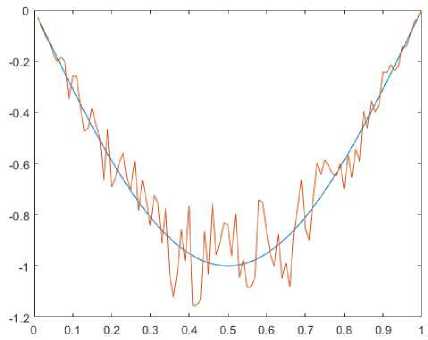
Fig. 1. The results of calculations of q1 with 25% noise and 6 = 0, 25. The results are displayed on Fig. 1 for the function q1 = sin(n(t + 1)). In this case Eq = 0, 24, Eu = 0, 091, ts = 32, 8. The calculation shows that the algorithm is stable with respect to the noise.

Table 1

T he results of experiments for the second group of the da ta

No	δ	q i	ε q	ε u	τ s
1	0,01	log(t + 1)	0,0061	0,0033	3,41
2	0,05	log(t + 1)	0,0185	0,007	3,46
3	0,1	log(t + 1)	0,0581	0,031	3,44
4	0,01	e t +1	0,044	0,24	3,65
5	0,05	e t +1	0,217	0,09	3,3
6	0,1	e t +1	0,398	0,19	3,33
7	0,01	sin(n(t + 1))	0,0091	0,0037	3,46
8	0,05	sin(n(t + 1))	0,037	0,015	3,25
9	0,1	sin(n(t + 1))	0,089	0,032	3,34

For the third group of experiments, we use an array of 8 points { y i } and the corresponding functions q i below. We also slightly change the mesh construction area by stretching and compressing it by 2 times relative to the X and Z axes, respectively. Let’s set the random noise to 5 percent. The results are exhibited in Table 2 and on Fig. 2. According to the results of computational experiments, it is clear that the calculation error increases as the coordinates of the overdetermination point move away from the lower face. The results shows good convergence of the algorithm as a whole.

Table 2

The resul	ts of experiments for the third group of the data
No	y i	q i	ε q i
1	(0,2;0,1;0,45)	sin(π(10t + 1)) - 16	2,44
2	(0,6;0,3;0,35)	(t - 2) 2 +16	1,39
3	(1;0,5;0,25)	(t - 1) 3 - 12	1,32
4	(1,4;0,7;0,35)	log 2 (0, 1t + 1) - 8	4,53
5	(0,2;0,9;0,05)	2t+ 12	0,72
6	(0,6;0,7;0,15)	- 10t - 1	0,31
7	(1,8;0,1;0,05)	- cos(π 10t) + 8	0,93
8	(1,4;0,3;0,15)	-e 2t+0,5 + 4	0,97

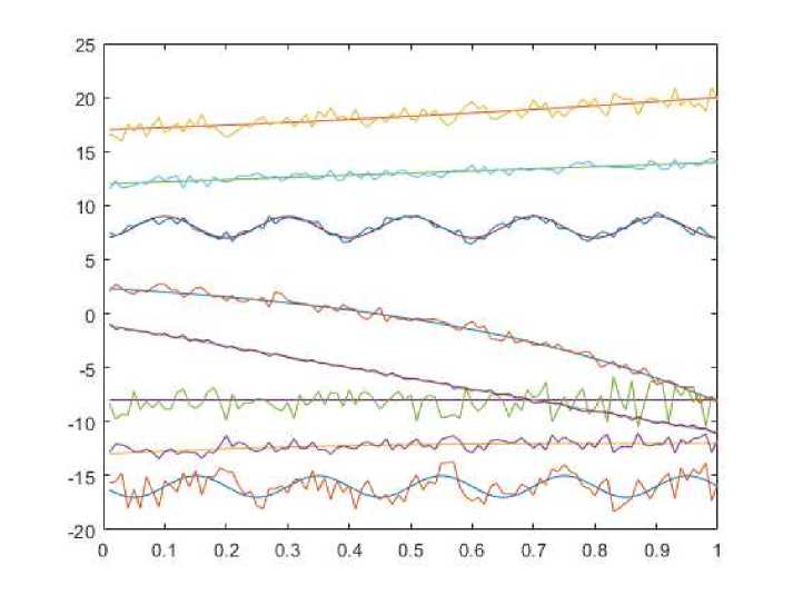
Fig. 2 . The results of calculations of q i with 5% noise

Conclusions

Using theoretical results on well-posedness of the problem, we construct a numerical algorithm for recovering the surface flow on the lower face with the use of point observations of the concentration. It is based on the conventional methods (in our case FEM and difference schemes). The results of numerical experiments are presented. The obtained results reveal the accuracy, efficiency, and robustness of the proposed algorithm. It is stable under random perturbations of the data.

Acknowledgments. This work was supported by the Russian Science Foundation and the Government of the Khanty-Mansiysk Autonomous Okrug-YUGRA (Grant no. 22-1120031).