The impact of feature selection techniques on the performance of predicting Parkinson’s disease

Автор: Abdullah Al Imran, Ananya Rahman, Humayoun Kabir, Shamsur Rahim

Журнал: International Journal of Information Technology and Computer Science @ijitcs

Статья в выпуске: 11 Vol. 10, 2018 года.

Бесплатный доступ

Parkinson’s Disease (PD) is one of the leading causes of death around the world. However, there is no cure for this disease yet; only treatments after early diagnosis may help to relieve the symptoms. This study aims to analyze the impact of feature selection techniques on the performance of diagnosing PD by incorporating different data mining techniques. To accomplish this task, identifying the best feature selection approach was the primary focus. In this paper, the authors had applied five feature selection techniques namely: Gain Ratio, Kruskal-Wallis Test, Random Forest Variable Importance, RELIEF and Symmetrical Uncertainty along with four classification algorithms (K-Nearest Neighbor, Logistic Regression, Random forest, and Support Vector machine) on the PD dataset collected from the UCI Machine Learning repository. The result of this study was obtained by taking the four different subsets (Top 5, 10, 15, and 20 features) from each feature selection approach and applying the classifiers. The obtained result showed that in terms of accuracy, Random Forest Variable Importance, Gain Ratio, and Kruskal-Wallis Test techniques generated the highest 89% score. On the other hand, in terms of sensitivity, Gain Ratio and Kruskal-Walis Test approaches produced the highest 97% score. The findings of this research clearly indicated the impact of feature selection techniques on predicting PD and our applied methods outperformed the state-of-the-art performance.

Еще

Parkinson’s Disease, Feature selection, Feature ranking technique, Classification, Data Mining, Accuracy, Sensitivity

Короткий адрес: https://sciup.org/15016311

IDR: 15016311 | DOI: 10.5815/ijitcs.2018.11.02

Текст научной статьи The impact of feature selection techniques on the performance of predicting Parkinson’s disease

Published Online November 2018 in MECS DOI: 10.5815/ijitcs.2018.11.02

The Parkinson’s Disease (PD) is a progressive, and neurodegenerative brain disorder that affects predominately dopamine-producing (“dopaminergic”) neurons in a specific area of the brain called substantia nigra [1]. Sometimes PD can be genetic, however, in most of the cases, it does not seem to run in families. Some experts believe that exposure to chemicals in the environment might be a factor behind PD. The prevalence of Parkinson’s disease increases with an average age of 62, where 15% of those diagnosed are under 50 which is known as “Young-Onset PD” [3]. People with PD usually experiences four key symptoms - Tremor (shaking), Bradykinesia (slowness of movement), Rigidity (stiffness), Postural Instability (difficulty with balance) [3]. These symptoms begin to grow gradually on the one side of the body and affect both sides at some time. Approximately 60,000 Americans are diagnosed with PD each year while more than 10 million people worldwide are living with PD [2]. Diagnosing PD is a challenging task as there is no lab test for PD. However, doctors take the help of medical history and neurological screen tests to diagnose it. Unfortunately, there is no cure for PD till now. However, after early diagnosis, treatments can help to relieve the symptoms. So it is vital to diagnose PD as early as possible.

Nowadays, the modern medical equipments generate a large amount of health data, which can play a very important role in diagnosing diseases. Previously, many researchers in the biomedical and health sector have proved that by utilizing the health data with modern data mining techniques, it is possible to recognize the diseases more accurately. In case of PD, several screening tests are used for diagnosis purposes. These tests produce a huge amount of data which make it possible now to predict PD up to a certain accuracy with the help of data mining techniques. For instance, a tele-monitoring device was used to record speech signals and in [5] Tsanas et al. applied different linear and nonlinear regression methods over the tele-monitoring dataset to score on the UPDRS scale and predict the clinician's symptoms for PD. N. Monami et al. [6] used a probability density function based algorithm named ensemble average propagator (EAP) to classify PD people from the diffusion MRI (dMRI) dataset. However, there exists plenty of research gaps in applying data mining techniques for diagnosing PD with higher accuracy.

The dataset on PD from the UCI machine learning repository is a popular dataset to the data mining researchers that provides a range of biomedical voice measurements from 31 people, where 23 people have PD [4]. There are numerous researchers who have used different data mining techniques on this dataset and achieved very significant accuracy in classifying PD. Most of the researchers worked on discovering the best classification model. However, to the best of the authors knowledge, no prominent work has been done on feature selection for this dataset.

To overcome the research gap identified above, this paper aims to find the best feature selection technique for PD dataset from the perspective of data mining and statistics. Identifying the best feature selection technique will certainly accelerate the accuracy of PD diagnosis, produce more reliable diagnosis decision and optimize the computational power. For achieving this goal, as a first step, we acquired the PD dataset from UCI machine learning repository, trimmed and renamed the features and performed some descriptive statistical analysis to check the missing values and dealt with imbalanced class. The main contributions of this paper are:

1) Tackled the imbalanced class problem of the dataset with SMOTE technique.
2) Identified the best feature selection approach for predicting PD and presented the impact by a comparative analysis with the state-of-the-art

methods.

II. Related Works

Previously, a significant number of researchers had worked on classifying of PD using data mining techniques. Most of those works were aimed to increase the accuracy and identify the best methods by applying a number of classification algorithms and statistical methods.

Salama, Aida et al. [7] evaluated the performance of three classifiers - Decision Tree, Naïve Bayes, and Neural Network. Among all of these three classifiers, Decision Tree produced the highest accuracy of 91.63%. They used 10-Fold Cross Validation to measure the classification accuracy. As for future work, they recommend to perform feature selection and apply these three classifiers on the best-chosen features to improve the accuracy.

Salim et al. [8] implemented seven machine learning methods and examined the effectiveness and performance of those techniques. They used 10-Fold Cross Validation and seven other statistical measures to evaluate the performance. They also used t-tests to evaluate the statistical significance of the results. They concluded that SVM achieved the highest performance the accuracy of 92%. They would like to work on feature selection in future.

Dr. R. Geetha and G. Sivagami [9] executed a comparative study of 13 different classification algorithms. They used feature relevance analysis and the accuracy analysis to come up with the best classification algorithm. They tried numerous feature selection algorithms where they found Fisher filtering as a good feature ranking system. As training dataset, they used the whole dataset which included 197 instances with 22 characteristic features. However, they did not specify if they used test-train split or cross-validation. Although, they found the Random Tree Algorithm as the best classifier with an accuracy of 100%, however, our analysis found that they used the same dataset for training and testing the classification models which made their results biased. They wanted to extend their work in classifying PD from the Parkinson tele-monitoring dataset.

Resul Das [10] compared four independent classification methods (Neural Networks, DMneural, Regression and Decision Tree) to find the most efficient method for distinguishing healthy individuals from PD affected people. They created mutually exclusive datasets by randomly partitioning the input dataset into train and validation datasets. They found neural network classifier producing the best result. The overall classification score for the neural network classifier was 92.9%. They also compared their scores with the score of kernel support vector machines. However, they have not used any intensive feature selection methods.

Tarigoppula et al. [11] worked on understanding the factors responsible for Parkinson Disease. They did a comparative experiment on two datasets, one was the dataset from UCI ML repository which had 24 attributes and fundamental frequency values whereas another dataset was collected by their own having three attributes.

For their own dataset, they collected voice data from PD affected and healthy people who crossed 40 years of age. The collected dataset contained three attributes, named Frequency (F), Modulation (M) and Phase or Impendence (I). They used the Rank Search Method on the dataset of UCI ML repository and found Flo, Spread1, and APQ as the best three attributes for classifying the PD people. Afterward, they applied four classifiers (Bayes Net, Logistics, Simple Logistics, and Random Forest) on both of the datasets and compared the results where they found Logistics method yielding the highest result of 100% for both of the datasets.

Arvind Kumar [12] used the minimum redundancy maximum relevance (MRMR) feature selection algorithm to select the most important features and applied 8 different data mining methods on the dataset. His aim was to find out the best performing classifier after selecting features by MRMR algorithm. Among all the 23 features he selected top 5, 8, 10, and 20 features by using MRMR algorithm. Then he used each of those data subsets over 8 different classifiers and found that the random forest classifier with 20 number of features selected by MRMR produced the highest overall accuracy 90.3%, precision 90.2%, Mathews correlation coefficient values of 0.73 and ROC values 0.96.

Satish M. Srinivasan et al. [13] performed another research to demonstrate how the three different pre-processing techniques (Discretization, Resampling, and SMOTE) influence the results in improving the prediction accuracies of an ANN-based (Multi-Layer Perceptron) classifier on the PD dataset. Each time they took a different pre-processing technique and applied to the dataset. After pre-processing, they partitioned the dataset into training and testing datasets in two different ratios (80:20 and 70:30). They also used 10-fold cross-validation on the entire dataset. They performed 36 different experiments involving 12 different pre-processing techniques. After analyzing all the experimental results, they found that the 70:30 split over the combination of the pre-processing techniques named Resampling and SMOTE yielded the highest prediction accuracy for the ANN-based (MLP) classifier. In future, they want to extend their work to understand if the three different pre-processing techniques all combined, separately, or in any combination improve the prediction accuracy for a variety of supervised classifiers.

Marius Ene [14] used three types (IS, MCS and HS) of probabilistic neural networks (PNN) to classify the healthy people from the PD people. 70% of the dataset was used for the training and the rest of 30% was used for testing. The PNN model was used 10 times for each method (IS, MCS or HS), and the results were averaged across 10 computer run. All the methods produced accuracies between 79% to 81%. In future, Marius wants to improve the search technique focusing on different heuristic methods and analyze the PNN performances with other neural network types, such as MLP, RBF.

David Gil and Magnus Johnson [15] proposed a hybrid system combining ANN and SVM classifiers to assist the specialist in the diagnosis of Parkinson's Disease which showed a high accuracy of around 90%. The optimal solution for this layer was found to be 13 neurons. They used 6 measures (classification accuracy, sensitivity, specificity, positive predictive value, negative predictive value and a confusion matrix) to evaluate the system. They found outliers in the dataset and the dataset was imbalanced which directly affected the classification performance. There were 147 instances with PD and 48 healthy ones. They mentioned that the accuracy will be improved by eliminating the outliers from both the minority and majority classes and increasing the size of the minority class to the same size of the majority class.

Indira and Mehmet [16] used a combination of fuzzy c-means (FCM) clustering and pattern recognition methods on Parkinson’s disease dataset to distinguish between healthy people and PD people. They applied correlation filter (correlation coefficient > 0.95) to the 23 attributes from where 12 features were removed and the rest 11 features were selected. In the first part of their experiment, they applied FCM clustering on the dataset and because of the imbalanced dataset they achieved a success rate of 58.46%. In the second part of their experiment, they used the equal number of train-test data for the FCM and pattern recognition model which improved the success rate for and also handled the effect of imbalanced class. The best result they achieved was in the positive predicted value which was 80.88 %.

Shamli et al. [30] proposed a big data based predictive analytics framework with a combination of three different data mining techniques namely: Artificial Neural Network (ANN), Decision tree (DT), and Support Vector Machines (SVM) to gain insights from the tele-monitoring voice dataset of Parkinson's disease affected patients. They have used accuracy, sensitivity, and specificity for evaluating their results. The found that when the Population (Milllion) size is larger the performance of the models are better. The highest accuracy and sensitivity they obtained was 91% and 97% respectively which were produced by the ANN classifier. They obtained these highest results when they took population size as 3.0 million. They had not applied any feature selection techniques.

From the above discussion, we can conclude that, research gap still exists for classifying PD more efficiently and accurately. We have identified that in most of the cases feature selection and the imbalanced class problem were overlooked. The modern data mining methodology proves that feature selection techniques can be used to accelerate the model accuracy, efficiency and save computational power. Moreover, the performance of the classifiers should not be measured by only using accuracy but with other metrics especially when the data is imbalanced.

III. Description of Dataset

Previously, many researchers had used a different number of datasets to classify Parkinson disease. Some of the well-known datasets were built from voice measurements, tele-monitoring device and MRI images.

Among all of these, voice measurement data achieved remarkable results in classifying Parkinson Disease. In [10], Resul Das mentioned that about 90% of people with Parkinson’s disease show some kind of vocal deteriorations. Hence, we have chosen a dataset for our research which was mainly composed of different vocal measurements and speech signals.

We collected the dataset [17] from the UCI Machine Learning Repository. This dataset was composed of a range of biomedical voice measurements from 31 people in which 23 people were affected with Parkinson's disease (PD). There are 24 attributes in the dataset in which each column contains a particular voice measurement except the “name” attribute. There are in total 195 rows in the dataset and each row contains an instance corresponding to one voice recording. There are around six voice recordings per patient. The main aim of the dataset is to distinguish the healthy people from PD people, according to the “status” column where 0 was set for healthy and 1 for PD. Table 1 presents the description of the columns excluding the “name” column-

Table 1. Description of columns

No.	Feature Name	Description
1	MDVP Fo (Hz)	Average vocal fundamental frequency
2	MDVP Fhi (Hz)	Maximum vocal fundamental frequency
3	MDVP Flo (Hz)	Minimum vocal fundamental frequency
4	MDVP Jitter (%)	MDVP jitter as percentage
5	MDVP Jitter (Abs)	MDVP jitter as absolute value in microseconds
6	MDVP RAP	MDVP Relative Amplitude Perturbation
7	MDVP PPQ	MDVP Period Perturbation Quotient
8	Jitter DDP	Difference of differences between cycles, divided by the average period
9	MDVP Shimmer	MDVP local shimmer
10	MDVP Shimmer (dB)	MDVP local shimmer in decibels
11	Shimmer: APQ3	3 Point Amplitude Perturbation Quotient
12	Shimmer: APQ5	5 Point Amplitude Perturbation Quotient
13	MDVP: APQ	MDVP Amplitude Perturbation Quotient
14	Shimmer: DDA	Average absolute difference between consecutive differences and the amplitude of consecutive periods
15	NHR	Noise to Harmonic Ratio
16	HNR	Harmonics to Noise Ratio
17	RPDE	Recurrence Period Density Entropy
18	DFA	Detrended Fluctuation Analysis
19	Spread1	Non Linear measure of fundamental frequency
20	Spread2	Non Linear measure of fundamental frequency
21	D2	Correlation Dimension
22	PPE	Pitch Period Entropy
23	Status	Health Status: 1 - Parkinson, 0 - Healthy

All the columns presented above contain real numerical values. There are no missing values in the dataset. Table 2 shows some descriptive statistical analysis for each attribute.

Fig. 1 demonstrates the distribution of classes for the feature “status” which contains the classes (Healthy (0) and PD (1).

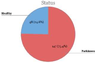
Fig.1. Distribution of classes.

From Fig. 1, we can see that in this dataset, among 195 instances, there were 147 instances with PD and only 48 instances with healthy people. That means, only 24.6% people are labeled as healthy and the rest 75.4% people are labeled with PD which arises the class imbalance problem for this dataset. Therefore, if we classify all the instances as PD, still we would get 75.4% accuracy.

IV. Methodology

To start working with the dataset, firstly, we renamed all the 24 columns and reordered all of them. Secondly, we omitted the unnecessary column - “name”, which contained the names of the patients. We finalized the dataset with 23 columns. Thirdly, we performed descriptive statistical analysis on the processed dataset to understand it more precisely. After performing all the three starting steps, we started performing our main activities.

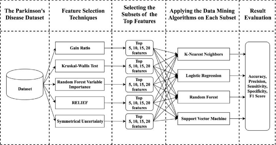
The main activities that we performed in this work were- ranking the features, balancing and partitioning the dataset, selecting the feature subsets, classification, and evaluation. All of the activities are described in the following subsections. All the implementations and experiments were performed using the R programming environment [18]. Figure 2 represents the overall workflow of this study.

A. Ranking the features

We have used five popular statistical and data mining based techniques to calculate the feature importance and ranked all the features of the dataset according to their respective score of importance. The five techniques are -i) Gain Ratio, ii) Kruskal-Wallis Test, iii) Random Forest Variable Importance, iv) RELIEF and v) Symmetrical Uncertainty. All the five techniques are detailed below with their ranking scores for each feature. We used the “mlr” [19] package to calculate the feature importance scores and rank the features.

i) Gain Ratio:

The Gain ratio is an improved version of the information gain that was used in the C4.5 algorithm [20]. It measures how much information a feature gives about the targeted feature. The information gain used in the ID3 algorithm has a preference for selecting features that have a large number of values. Gain ratio uses a kind of normalization technique to the information gain to overcome this bias. It normalizes information gain by the “intrinsic information” of a split, which is defined as the information need to determine the branch to which an instance belongs. The intrinsic information value represents the potential information generated by splitting the training data set D into v partitions, corresponding to v outcomes on attribute A.

IntrinsicInfo(D) =

v¹ DI |Dj|

StT^^’

The gain ratio is defined as:

Gam(A) IntrinsicInfo(A)

Dataset

The Parkinson's Disease Dataset

Feature Selection Techniques

Result Evaluation

। Applying the Data Mining । Algorithms on Each Subset

Selecting the Subsets of the

Top Features

♦

Accuracy, Precision, Sensitivity, Specificity, Fl Score

Gain Ratio

Kruskal-Wallis Test

К-Nearest Neighbors

Random Forest

Support Vector Machine

Logistic Regression

RELIEF

Symmetrical Uncertainty

Random Forest Variable Importance

' Top '

5,10,15, 20 features _v

Top 5,10,15,20 _v features _v

' Top ' 5,10,15,20 features

Top 5,10, 15,20 v features

Top

5,10,15,20 features ,

Fig.2. The overall workflow

Table 2. Descriptive statistical analysis for each attribute

Feature	Min.	1st.Qu.	Median	Mean	3rd.Qu.	Max.	S.D.
MDVP.FoHz	88.333	117.572	148.79	154.228641	182.769	260.105	41.39006475
MDVP.FhiHz	102.145	134.8625	175.829	197.1049179	224.2055	592.03	91.49154764
MDVP.FloHz	65.476	84.291	104.315	116.3246308	140.0185	239.17	43.52141318
MDVP.Jitter	0.00168	0.00346	0.00494	0.006220462	0.007365	0.03316	0.004848134
MDVP.JitterAbs	0.000007	0.00002	0.00003	4.40E-05	0.00006	0.00026	3.48E-05
MDVP.RAP	0.00068	0.00166	0.0025	0.00330641	0.003835	0.02144	0.002967774
MDVP.PPQ	0.00092	0.00186	0.00269	0.003446359	0.003955	0.01958	0.002758977
Jitter.DDP	0.00204	0.004985	0.00749	0.009919949	0.011505	0.06433	0.008903344
MDVP.Shimmer	0.00954	0.016505	0.02297	0.029709128	0.037885	0.11908	0.018856932
MDVP.ShimmerdB	0.085	0.1485	0.221	0.282251282	0.35	1.302	0.19487729
Shimmer.APQ3	0.00455	0.008245	0.01279	0.015664154	0.020265	0.05647	0.010153162
Shimmer.APQ5	0.0057	0.00958	0.01347	0.017878256	0.02238	0.0794	0.012023706
MDVP.APQ	0.00719	0.01308	0.01826	0.024081487	0.0294	0.13778	0.016946736
Shimmer.DDA	0.01364	0.024735	0.03836	0.046992615	0.060795	0.16942	0.030459119
NHR	0.00065	0.005925	0.01166	0.024847077	0.02564	0.31482	0.040418449
HNR	8.441	19.198	22.085	21.88597436	25.0755	33.047	4.425764269
RPDE	0.25657	0.421306	0.495954	0.498535538	0.5875625	0.685151	0.103941714
DFA	0.574282	0.6747575	0.722254	0.718099046	0.7618815	0.825288	0.05533583
Spread1	-7.964984	-6.450096	-5.720868	-5.684396744	-5.046192	-2.434031	1.090207764
Spread2	0.006274	0.1743505	0.218885	0.226510349	0.279234	0.450493	0.083405763
D2	1.423287	2.0991255	2.361532	2.381826087	2.636456	3.671155	0.382799047
PPE	0.044539	0.137451	0.194052	0.206551641	0.25298	0.527367	0.090119322
Status	0	1	1	0.753846154	1	1	0.431878034

ii) Kruskal-Wallis Test:

The Kruskal-Wallis test [21] is a non-parametric statistical technique that measures the significant differences on a continuous dependent variable by a categorical independent variable. The parametric equivalent to this test is the one-way analysis of variance (ANOVA). The ANOVA test assumes that the dependent variable is normally distributed and there is approximately equal variance whereas the Kruskal-Wallis test does not assume that the data come from a distribution with approximately equal variance. The Kruskal-Wallis test is defined by the following steps:

Step 1: Sort the data for all groups/samples into ascending order in one combined set.

Step 2: Assign ranks to the sorted data points. Give tied values the average rank.

Step 3: Add up the different ranks for each sample.

Step 4: Calculate the H statistic:

[ 12 v Г/1

H = —--— > — -3(n+1)

n(n + 1)4^ Hj where, n = sum of sample sizes for all samples, c = number of samples,

Tj = sum of ranks in the j^th sample, n.j = size of the j^th sample.

Step 5: Find the critical chi-square value, with c-1 degrees of freedom.

Step 6: Compare the H value from Step 4 to the critical chi-square value from Step 5.

If the critical chi-square value is less than the H statistic, reject the null hypothesis that the medians are equal. If the chi-square value is not less than the H statistic, there is not enough evidence to suggest that the medians are unequal.

iii) Random Forest Variable Importance:

Random Forest [22] is a tree-based learning algorithm that uses an ensemble of decision trees. It generates a list of predictor variables with a corresponding importance score for each variable. This score is used in ranking the features that are significant in predicting the results. For calculating the variable importance from the ensembles of randomized trees, Breiman (2001, 2002) proposed to evaluate the importance of a variable X_m for predicting Y by adding up the weighted impurity decreases p(t)M(s_t,t) for all nodes t where X _m is used, averaged over all N_T trees in the forest:

Imp⁽X) = 1-^ ^ p⁽t)M(St,t)

T T teT:v(st)=Xm where p(t) is the proportion Nt/N of samples reaching t and v(st) is the variable used in split st.

iv) RELIEF:

Kira and Rendell [23-24] developed the Relief algorithm which was inspired by instance-based learning. Relief measures a feature score for each feature that can be used to estimate feature relevance to the target result. This score can be used to rank and select top scoring features for feature selection. The feature score has a range from -1 (worst) to +1 (best). The algorithm is defined as follows:

For a data set with n instances and p features, belonging to two known classes. The algorithm will be repeated m times starting with a p-long weight vector (W) of zeros. At each iteration, the feature vector (X) belonging to one random instance, and the feature vectors of the instance closest to X are taken. The closest distance is calculated by the Euclidean distance formula from each class. The closest same-class instance is called 'near-hit', and the closest different-class instance is called 'near-miss'. Then it updates the weight vector such that,

W_t = W_t- (X_f - nearHit_t)² + (X_t - nearMiss_t)²

Thus the weight of any given feature decreases if it differs from that feature in nearby instances of the same class more than nearby instances of the other class, and increases in the reverse case. After m iterations, divide each element of the weight vector by m. This becomes the relevance vector. Features are selected if their relevance is greater than a threshold τ.

v) Symmetrical Uncertainty:

Symmetrical Uncertainty a normalized form of the Mutual Information which was introduced by Witten and Frank, 2005 [25]. It measures how much information is shared between the feature values and target classes by utilizing the measure of correlation. The mutual information between two discreet random variables A and B jointly distributed according to p(A, B) is given by:

Z p(A,B)

Hence, the Symmetrical Uncertainty is defined by the following equation:

SU(A,B) = 2 .

Ml(A.B') H(A) + H(B)

Here, H(X) is the Entropy of set random variable X.

B. Partitioning and Balancing the dataset

At first, we partitioned the actual dataset into a test set and a training set. The test set contained 30% and the training set contained 70% of the actual dataset. In the description of the dataset section, we have mentioned that this dataset has class imbalance problem.

After partitioning the dataset both of the datasets still contain the same class imbalance problem. To maintain the maximum authenticity of the actual data, we applied the Synthetic Minority Oversampling Technique (SMOTE) [26] on the training set only and kept the test set unchanged as the real world data won't be always balanced. SMOTE is a popular oversampling technique that was proposed to improve random oversampling. Previously many researchers used this technique on health data and found significant positive results. After balancing the training set using SMOTE, there were 99 instances with the status “healthy” and 104 instances with the status “PD”.

C. Selecting the Feature Subsets

As our prime focus was examining the impact of different feature ranking algorithms, we did not subset the features using traditional forward selection or backward elimination techniques. Rather, we din subset the features by taking top 5, 10, 15 and 20 features from every feature ranking algorithms. This approach of making subsets of features made our experiment and analysis less complex.

D. Classification

For classification purpose, we chose four different classification algorithms from different categories –

i) K-Nearest Neighbors (KNN):

KNN [27] is a distance-based classification algorithm that uses a distance function to compute the distances between the entities to classify an entity according to its K number of closest entities. The most prominent distance functions it uses are Euclidean distance and the Manhattan distance. It makes the classification according to the majority of its K-nearest neighbors in the feature space.

ii) Logistic Regression:

Logistic regression [28] is a nonlinear parametric regression algorithm that uses a logistic function to measure the relationship between the features and the target. Logistic regression is ideal for the classification tasks where the target variable is binary and the features are either continuous or categorical.

iii) Random Forest:

Random Forest [22] is an advanced type of classification algorithm based on decision tree. It uses random selection for features to build a forest of decision trees and combines a group of decision trees which is generated by performing a random selection of sample data and features at each node that will be split. The splitting operation is performed mostly by using Gain Ratio, Information Gain or Gini Index. Finally, generates a set of decision trees at training time and each of the generated trees outputs a relevant class.

iv) Support Vector Machine (SVM):

SVM [29] is a kernel-based non-parametric classification algorithm that is basically effective for the classification problems. It transforms the original data into a higher dimension, from where it can find a hyperplane for data separation using essential training tuples called support vectors. Therefore, the best hyperplane should have the largest margin of separation between both of the classes.

E. Evaluation

We have used 5 different evaluation metrics for evaluating the classification results. The evaluation metrics are–

i) Accuracy - _ TP+TN — TP+TN+FP+FN TP ii) Precision : — TP+FP iii) Sensitivity or Recall — TP+FN iv) Specificity TN — TN+FP v) F1 Score = 2 (precision. recall) (precision + recall) where, TP, TN, FP and FN are derived from the confusion matrix.

For result analysis and visualization, we have mainly used the accuracy and sensitivity measure. Since, this is a disease classification problem, sensitivity is a very important metric for this problem as it tells us what proportion of patients that actually had Parkinson's disease and was diagnosed by the classifier as having the disease. On the other hand, the accuracy metric is important as it tells us the number of correct predictions made by the classifier among all kinds of predictions made. We have included all of our findings for each evaluation metrics in the appendix section.

V. Result Analysis

The primary focus of this paper is to analyze and compare the impact of five different feature ranking techniques over four different classification algorithms for this particular dataset. In the methodology section, we have described the five feature ranking techniques that have been used in this feature ranking experiment.

Table 3 shows the final result that was obtained by each feature ranking technique. All the features were ranked according to their importance score computed by their respective techniques. The more detailed tables for each feature ranking techniques with all computed scores are attached in the appendix section.

From table 3, we took subsets of top 5, 10, 15 and 20 features from each technique and applied four classification algorithms (KNN, Logistic Regression, Random Forest, and SVM) on each subset of features. As we mentioned in the evaluation subsection under the methodology section that, we considered “accuracy” and “sensitivity” metric to analyze, visualize and compare the performance of the models.

Table 3. Feature Ranking results for each ranking technique

Rank	Gain Ratio	Kruskal-Wallis Test	Random Forest Variable Importance	RELIEF	Symmetrical Uncertainty
1	MDVP.FloHz	Spread1	PPE	Spread1	PPE
2	Spread1	PPE	MDVP.FoHz	PPE	MDVP.FloHz
3	MDVP.APQ	MDVP.APQ	Spread1	Spread2	Spread1
4	PPE	Spread2	Spread2	DFA	MDVP.APQ
5	NHR	MDVP.JitterAbs	MDVP.FhiHz	RPDE	MDVP.FoHz
6	Spread2	MDVP.PPQ	MDVP.FloHz	MDVP.FoHz	MDVP.Shimmer
7	MDVP.FhiHz	MDVP.ShimmerdB	MDVP.APQ	MDVP.FloHz	MDVP.JitterAbs
8	MDVP.RAP	MDVP.Shimmer	RPDE	HNR	Shimmer.APQ5
9	Jitter.DDP	MDVP.Jitter	MDVP.Shimmer	Shimmer.APQ3	MDVP.FhiHz
10	MDVP.Shimmer	Jitter.DDP	MDVP.JitterAbs	Shimmer.DDA	Spread2
11	Shimmer.APQ5	MDVP.RAP	Shimmer.APQ5	MDVP.Shimmer	MDVP.RAP
12	MDVP.ShimmerdB	NHR	Shimmer.APQ3	Shimmer.APQ5	Jitter.DDP
13	MDVP.FoHz	Shimmer.APQ5	HNR	MDVP.PPQ	MDVP.ShimmerdB
14	Shimmer.APQ3	Shimmer.APQ3	MDVP.RAP	MDVP.JitterAbs	NHR
15	Shimmer.DDA	Shimmer.DDA	Shimmer.DDA	MDVP.RAP	Shimmer.APQ3
16	MDVP.JitterAbs	HNR	Jitter.DDP	Jitter.DDP	Shimmer.DDA
17	MDVP.PPQ	D2	DFA	MDVP.ShimmerdB	MDVP.PPQ
18	MDVP.Jitter	RPDE	MDVP.ShimmerdB	MDVP.Jitter	MDVP.Jitter
19	HNR	MDVP.FoHz	D2	MDVP.APQ	HNR
20	RPDE	MDVP.FloHz	MDVP.PPQ	MDVP.FhiHz	RPDE
21	D2	MDVP.FhiHz	MDVP.Jitter	D2	D2
22	DFA	DFA	NHR	NHR	DFA

Fig. 3. shows a comparative analysis of the accuracy metric for different classification algorithms for the four different subsets of five feature selection techniques.

From Fig. 3, we find that the SVM classifier yields the highest accuracy of 0.89 with the subset of top 5 features, taken from the Random Forest Variable Importance technique. If we consider a faster learning algorithm than SVM (as SVM is a lazy learner) then, the logistic regression algorithm yields the highest accuracy of 0.89 by taking the subset of top 10 features from both Gain Ratio and Kruskal-Wallis Test technique. Here we also find the RELIEF technique performs the worst in terms of accuracy metric.

Fig. 4. shows a comparative analysis of the sensitivity metric for different classification algorithms for the four different subsets of five feature selection techniques.

From Fig. 4, we find that both Random Forest and

Logistic Regression classifier outputs the highest sensitivity score of 0.97 by taking the subset of top 10 features from the Gain Ratio and Kruskal-Walis Test respectively. If we consider the faster learning algorithm then, the Logistic Regression with top 10 features from the Kruskal-Walis Test will be the best. In the other hand, we also find that in overall case the Symmetrical Uncertainty technique performs the worst in terms of sensitivity score.

To clearly represent the impact of feature selection, we have made a comparative visualization of the state-of-the-art methods with the methods used in this study. Fig. 5. shows the comparative analysis of the results of Shamli et al. [30] with the results of this study. The visualization represents the classifiers and evaluation metrics that were mutual in both of the studies.

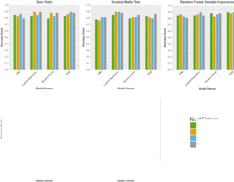
No. of Features

Top 5 Features

Top 10 Features

Top 15 Features

Top 20 Features

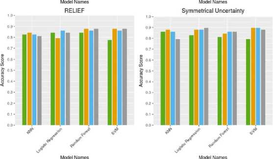
Fig.3. Comparative analysis of the accuracy metric for different classification algorithms.

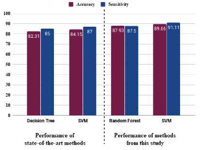
Fig.5. Performance comparison between stat-of-the-art methods and methods in this study

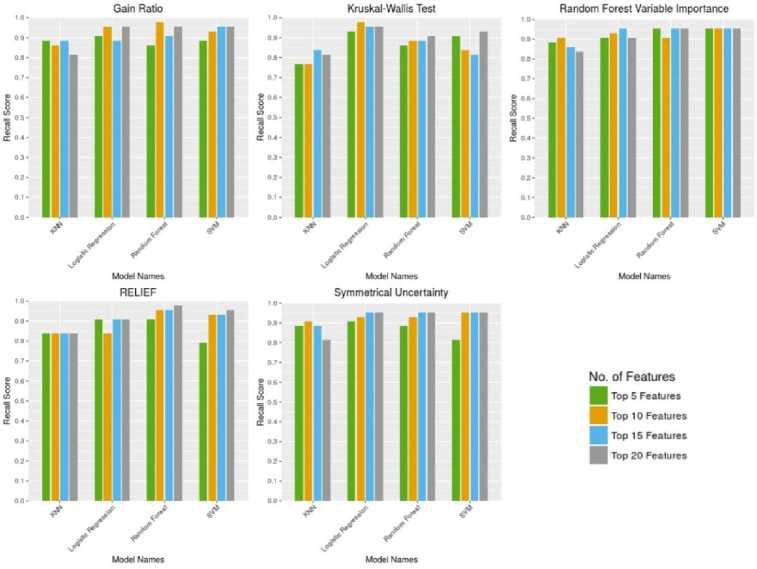
Fig.4. Comparative analysis of the sensitivity metric for different classification algorithms

In Figure 5, we have taken the performance of Decision Tree and SVM from [30] which were performed without any feature selection. On the other hand, we have taken the performance of Random forest and SVM from this study which was trained by selecting top 10 and 15 features respectively. The figure clearly shows that, the classifiers with feature selection overtakes the state-of-the-art methods which did not used any feature selection techniques.

The primary advantage and novelty of this study are:

• This study reveals the impact of different feature selection techniques for diagnosing Parkinson’s disease which can be used to improve the accuracy of the model. Thus, the diagnosis will be more accurate and reliable.
• The feature selection techniques rank all the features according to the importance level and thus the minimal number of features can be selected for

training the models, and obtaining the best performance from the models. It will save a lot of computational power and increase diagnosing efficiency.

All the detailed tables for the classification algorithms with all five metrics are attached in the appendix section.

VI. Conclusion and Future Work

Classification of Parkinson’s disease is one of the most challenging and important problems in the biomedical engineering research. Though many significant works had been performed by many prominent researchers, there still exists a research gap in improving the classification performance. In our paper, we showed the impact of five different feature ranking techniques in improving the classification performance. We analyzed the Gain Ratio, Kruskal-Walis Test, Random Forest Variable Importance, RELIEF and Symmetrical Uncertainty feature ranking techniques over KNN, Logistic Regression, Random Forest and SVM classifiers and found a significant impact in the improvement of accuracy and sensitivity score. We found Random Forest Variable Importance, Gain Ratio, Kruskal-Wallis Test as the best impactful feature ranking techniques and the Logistic Regression, Random Forest and, SVM as the best performing classifiers for this particular dataset. On the other hand, we also found RELIEF and Symmetrical Uncertainty techniques as the worst impactful ranking technique and KNN as the worst performing classifier for this dataset.

Our future work can be extended to try other classifiers using the best feature ranking technique. We also want to work on handling the outliers and normalization.

Appendix A Model Performance for Gain Ratio

		Accuracy	Precision	Sensitivity	Specificity	F1-Score
Top 5 Features	KNN	0.8448276	0.7333333	0.9047619	0.8837209	0.8941176
	Logistic Regression	0.8275862	0.6	0.8666667	0.9069767	0.8863636
	Random Forest	0.7931034	0.6	0.8604651	0.8604651	0.8604651
	SVM	0.8275862	0.6666667	0.8837209	0.8837209	0.8837209
Top 10 Features	KNN	0.8275862	0.7333333	0.902439	0.8604651	0.8809524
	Logistic Regression	0.8965517	0.7333333	0.9111111	0.9534884	0.9318182
	Random Forest	0.8793103	0.6	0.875	0.9767442	0.9230769
	SVM	0.862069	0.6666667	0.8888889	0.9302326	0.9090909
Top 15 Features	KNN	0.862069	0.8	0.9268293	0.8837209	0.9047619
	Logistic Regression	0.8448276	0.7333333	0.9047619	0.8837209	0.8941176
	Random Forest	0.8275862	0.6	0.8666667	0.9069767	0.8863636
	SVM	0.8965517	0.7333333	0.9111111	0.9534884	0.9318182
Top 20 Features	KNN	0.7931034	0.7333333	0.8974359	0.8139535	0.8536585
	Logistic Regression	0.8965517	0.7333333	0.9111111	0.9534884	0.9318182
	Random Forest	0.8793103	0.6666667	0.8913043	0.9534884	0.9213483
	SVM	0.8793103	0.6666667	0.8913043	0.9534884	0.9213483

Appendix B Model Performance for Kruskal-Wallis Test

		Accuracy	Precision	Sensitivity	Specificity	F1- Score
Top 5 Features	KNN	0.7758621	0.8	0.9166667	0.7674419	0.835443
	Logistic Regression	0.8448276	0.6	0.8695652	0.9302326	0.8988764
	Random Forest	0.7931034	0.6	0.8604651	0.8604651	0.8604651
	SVM	0.8275862	0.6	0.8666667	0.9069767	0.8863636
Top 10 Features	KNN	0.7586207	0.7333333	0.8918919	0.7674419	0.825
	Logistic Regression	0.8965517	0.6666667	0.893617	0.9767442	0.9333333
	Random Forest	0.8103448	0.6	0.8636364	0.8837209	0.8735632
	SVM	0.8103448	0.7333333	0.9	0.8372093	0.8674699
Top 15 Features	KNN	0.8103448	0.7333333	0.9	0.8372093	0.8674699
	Logistic Regression	0.8965517	0.7333333	0.9111111	0.9534884	0.9318182
	Random Forest	0.8103448	0.6	0.8636364	0.8837209	0.8735632
	SVM	0.7931034	0.7333333	0.8974359	0.8139535	0.8536585
Top 20 Features	KNN	0.8103448	0.8	0.9210526	0.8139535	0.8641975
	Logistic Regression	0.8793103	0.6666667	0.8913043	0.9534884	0.9213483
	Random Forest	0.8448276	0.6666667	0.8863636	0.9069767	0.8965517
	SVM	0.862069	0.6666667	0.8888889	0.9302326	0.9090909

Appendix C Model Performance for Random Forest Variable Importance

		Accuracy	Precision	Sensitivity	Specificity	F1- Score
Top 5 Features	KNN	0.8448276	0.7333333	0.9047619	0.8837209	0.8941176
	Logistic Regression	0.8448276	0.6666667	0.8863636	0.9069767	0.8965517
	Random Forest	0.8793103	0.6666667	0.8913043	0.9534884	0.9213483
	SVM	0.8965517	0.7333333	0.9111111	0.9534884	0.9318182
Top 10 Features	KNN	0.862069	0.7333333	0.9069767	0.9069767	0.9069767
	Logistic Regression	0.862069	0.6666667	0.8888889	0.9302326	0.9090909
	Random Forest	0.8275862	0.6	0.8666667	0.9069767	0.8863636
	SVM	0.8793103	0.6666667	0.8913043	0.9534884	0.9213483
Top 15 Features	KNN	0.8275862	0.7333333	0.902439	0.8604651	0.8809524
	Logistic Regression	0.8965517	0.7333333	0.9111111	0.9534884	0.9318182
	Random Forest	0.862069	0.6	0.8723404	0.9534884	0.9111111
	SVM	0.8965517	0.7333333	0.9111111	0.9534884	0.9318182
Top 20 Features	KNN	0.8103448	0.7333333	0.9	0.8372093	0.8674699
	Logistic Regression	0.8448276	0.6666667	0.8863636	0.9069767	0.8965517
	Random Forest	0.8793103	0.6666667	0.8913043	0.9534884	0.9213483
	SVM	0.8793103	0.6666667	0.8913043	0.9534884	0.9213483

Appendix D Model Performance for RELIEF

		Accuracy	Precision	Sensitivity	Specificity	F1- Score
Top 5 Features	KNN	0.8275862	0.8	0.9230769	0.8372093	0.8780488
	Logistic Regression	0.8448276	0.6666667	0.8863636	0.9069767	0.8965517
	Random Forest	0.8448276	0.6666667	0.8863636	0.9069767	0.8965517
	SVM	0.7758621	0.7333333	0.8947368	0.7906977	0.8395062
Top 10 Features	KNN	0.8448276	0.8666667	0.9473684	0.8372093	0.8888889
	Logistic Regression	0.7931034	0.6666667	0.8780488	0.8372093	0.8571429
	Random Forest	0.8793103	0.6666667	0.8913043	0.9534884	0.9213483
	SVM	0.8793103	0.7333333	0.9090909	0.9302326	0.9195402
Top 15 Features	KNN	0.8275862	0.8	0.9230769	0.8372093	0.8780488
	Logistic Regression	0.862069	0.7333333	0.9069767	0.9069767	0.9069767
	Random Forest	0.862069	0.6	0.8723404	0.9534884	0.9111111
	SVM	0.862069	0.6666667	0.8888889	0.9302326	0.9090909
Top 20 Features	KNN	0.8103448	0.7333333	0.9	0.8372093	0.8674699
	Logistic Regression	0.8448276	0.6666667	0.8863636	0.9069767	0.8965517
	Random Forest	0.8793103	0.6	0.875	0.9767442	0.9230769
	SVM	0.8793103	0.6666667	0.8913043	0.9534884	0.9213483

Appendix E Model Performance for Symmetrical Uncertainty

		Accuracy	Precision	Sensitivity	Specificity	F1- Score
Top 5 Features	KNN	0.862069	0.8	0.9268293	0.8837209	0.9047619
	Logistic Regression	0.8275862	0.6	0.8666667	0.9069767	0.8863636
	Random Forest	0.8103448	0.6	0.8636364	0.8837209	0.8735632
	SVM	0.7931034	0.7333333	0.8974359	0.8139535	0.8536585
Top 10 Features	KNN	0.8793103	0.8	0.9285714	0.9069767	0.9176471
	Logistic Regression	0.8793103	0.7333333	0.9090909	0.9302326	0.9195402
	Random Forest	0.8448276	0.6	0.8695652	0.9302326	0.8988764
	SVM	0.8965517	0.7333333	0.9111111	0.9534884	0.9318182
Top 15 Features	KNN	0.862069	0.8	0.9268293	0.8837209	0.9047619
	Logistic Regression	0.8793103	0.6666667	0.8913043	0.9534884	0.9213483
	Random Forest	0.862069	0.6	0.8723404	0.9534884	0.9111111
	SVM	0.8965517	0.7333333	0.9111111	0.9534884	0.9318182
Top 20 Features	KNN	0.7931034	0.7333333	0.8974359	0.8139535	0.8536585
	Logistic Regression	0.8965517	0.7333333	0.9111111	0.9534884	0.9318182
	Random Forest	0.862069	0.6	0.8723404	0.9534884	0.9111111
	SVM	0.8793103	0.6666667	0.8913043	0.9534884	0.9213483

Appendix F Ranking for Gain Ratio with Score

Rank	Name of Feature	Score
1	MDVP.FloHz	0.39404636
2	Spread1	0.218968549
3	MDVP.APQ	0.215669838
4	PPE	0.210323859
5	NHR	0.197637014
6	Spread2	0.195129144
7	MDVP.FhiHz	0.191424377
8	MDVP.RAP	0.188081636
9	Jitter.DDP	0.188081636
10	MDVP.Shimmer	0.187832748
11	Shimmer.APQ5	0.182812303
12	MDVP.ShimmerdB	0.175315917
13	MDVP.FoHz	0.167519205
14	Shimmer.APQ3	0.16089819
15	Shimmer.DDA	0.16089819
16	MDVP.JitterAbs	0.159421402
17	MDVP.PPQ	0.15647848
18	MDVP.Jitter	0.14840726
19	HNR	0.109871083
20	RPDE	0.08442194
21	D2	0.078321375
22	DFA	0.072329204

Appendix G Ranking for Kruskal-Wallis Test with Score

Rank	Name of Feature	Score
1	Spread1	68.07581043
2	PPE	68.07581043
3	MDVP.APQ	45.88128144
4	Spread2	42.49421216
5	MDVP.JitterAbs	36.86811232
6	MDVP.PPQ	35.63484964
7	MDVP.ShimmerdB	35.11034876
8	MDVP.Shimmer	34.53463439
9	MDVP.Jitter	33.31708359
10	Jitter.DDP	33.24881094
11	MDVP.RAP	33.13133353
12	NHR	32.23731704
13	Shimmer.APQ5	31.47245818
14	Shimmer.APQ3	28.05109656
15	Shimmer.DDA	28.01978931
16	HNR	24.46065008
17	D2	21.85347251
18	RPDE	18.54647369
19	MDVP.FoHz	17.39775094
20	MDVP.FloHz	16.81299459
21	MDVP.FhiHz	13.2128627
22	DFA	9.694302721

Appendix H Ranking for Random Forest Variable Importance with Score

Rank	Name of Feature	Score
1	PPE	18.19753516
2	MDVP.FoHz	17.32143219
3	Spread1	16.24650385
4	Spread2	12.27959078
5	MDVP.FhiHz	11.37061638
6	MDVP.FloHz	10.86123423
7	MDVP.APQ	9.497221992
8	RPDE	8.938378359
9	MDVP.Shimmer	8.697315303
10	MDVP.JitterAbs	8.599481627
11	Shimmer.APQ5	8.303342552
12	Shimmer.APQ3	8.281248613
13	HNR	8.265140701
14	MDVP.RAP	8.083312777
15	Shimmer.DDA	8.041817596
16	Jitter.DDP	8.000576765
17	DFA	7.793754808
18	MDVP.ShimmerdB	7.723103178
19	D2	7.296279729
20	MDVP.PPQ	6.960939321
21	MDVP.Jitter	6.806083833
22	NHR	6.525867729

Appendix I Ranking for RELIEF with Score

Rank	Name of Feature	Score
1	Spread1	0.163583972
2	PPE	0.156309452
3	Spread2	0.136156445
4	DFA	0.105502737
5	RPDE	0.099031222
6	MDVP.FoHz	0.0963979
7	MDVP.FloHz	0.092323511
8	HNR	0.088754775
9	Shimmer.APQ3	0.080912943
10	Shimmer.DDA	0.080912826
11	MDVP.Shimmer	0.078018989
12	Shimmer.APQ5	0.074382632
13	MDVP.PPQ	0.070246517
14	MDVP.JitterAbs	0.067193676
15	MDVP.RAP	0.061936416
16	Jitter.DDP	0.061929684
17	MDVP.ShimmerdB	0.061643385
18	MDVP.Jitter	0.060984752
19	MDVP.APQ	0.054311969
20	MDVP.FhiHz	0.044894536
21	D2	0.040519132
22	NHR	0.026544228

Appendix J Ranking for Symmetrical Uncertainty with Score

Rank	Name of Feature	Score
1	PPE	0.28968762
2	MDVP.FloHz	0.286873536
3	Spread1	0.286180993
4	MDVP.APQ	0.237874754
5	MDVP.FoHz	0.228656764
6	MDVP.Shimmer	0.205369994
7	MDVP.JitterAbs	0.202753078
8	Shimmer.APQ5	0.202409095
9	MDVP.FhiHz	0.20098514
10	Spread2	0.200559957
11	MDVP.RAP	0.19934478
12	Jitter.DDP	0.19934478
13	MDVP.ShimmerdB	0.190487852
14	NHR	0.185443636
15	Shimmer.APQ3	0.175920657
16	Shimmer.DDA	0.175920657
17	MDVP.PPQ	0.166753857
18	MDVP.Jitter	0.153145443
19	HNR	0.1187121
20	RPDE	0.093036545
21	D2	0.086652278
22	DFA	0.076209263

Список литературы The impact of feature selection techniques on the performance of predicting Parkinson’s disease

http://parkinson.org/understanding-parkinsons/what-is-parkinsons, Last accessed at 9:00 PM on 29th March, 2018
http://parkinson.org/Understanding-Parkinsons/Causes-and-Statistics/Statistics, Last accessed at 11:00 AM on 3rd April, 2018
http://www.parkinsonsneurochallenge.org/sarasota-parkinsons-disease-resources/sarasota-what-is-parkinsons-disease.html, Last accessed at 10:00 PM on 9th April, 2018
Little, Max A., et al. "Exploiting nonlinear recurrence and fractal scaling properties for voice disorder detection." BioMedical Engineering OnLine 6.1 (2007): 23.
Tsanas, Athanasios, et al. "Accurate tele monitoring of Parkinson's disease progression by noninvasive speech tests." IEEE transactions on Biomedical Engineering 57.4 (2010): 884-893.
Tuite, Paul. "Brain Magnetic Resonance Imaging (MRI) as a Potential Biomarker for Parkinson’s Disease (PD)." Brain sciences 7.6 (2017): 68.
Mostafa, Salama A., et al. "Evaluating the Performance of Three Classification Methods in Diagnosis of Parkinson’s Disease." International Conference on Soft Computing and Data Mining. Springer, Cham, 2018.
Lahmiri, Salim, Debra Ann Dawson, and Amir Shmuel. "Performance of machine learning methods in diagnosing Parkinson’s disease based on dysphonia measures." Biomedical Engineering Letters 8.1 (2018): 29-39.
Ramani, R. Geetha, and G. Sivagami. "Parkinson disease classification using data mining algorithms." International journal of computer applications 32.9 (2011): 17-22.
Das, Resul. "A comparison of multiple classification methods for diagnosis of Parkinson disease." Expert Systems with Applications 37.2 (2010): 1568-1572.
Sriram, Tarigoppula VS, et al. "A Comparison And Prediction Analysis For The Diagnosis Of Parkinson Disease Using Data Mining Techniques On Voice Datasets." International Journal of Applied Engineering Research 11.9 (2016): 6355-6360.
Tiwari, Arvind Kumar. "Machine learning based approaches for prediction of Parkinson disease." Mach Learn Appl 3.2 (2016): 33-39.
Srinivasan, Satish M., Michael Martin, and Abhishek Tripathi. "ANN based Data Mining Analysis of the Parkinson’s Disease." International Journal of Computer Applications 168.1 (2017).
Ene, Marius. "Neural network-based approach to discriminate healthy people from those with Parkinson's disease." Annals of the University of Craiova-Mathematics and Computer Science Series 35 (2008): 112-116.
Gil, David, and Devadoss Johnson Manuel. "Diagnosing parkinson by using artificial neural networks and support vector machines." Global Journal of Computer Science and Technology 9.4 (2009).
Rustempasic, Indira, and Mehmet Can. "Diagnosis of parkinson’s disease using fuzzy c-means clustering and pattern recognition." Southeast Europe Journal of Soft Computing 2.1 (2013).
Little, Max A., et al. "Suitability of dysphonia measurements for tele monitoring of Parkinson's disease." IEEE transactions on biomedical engineering56.4 (2009): 1015-1022.
Team, R. Core. "R: A language and environment for statistical computing." (2013).
Bischl, Bernd, et al. "mlr: Machine Learning in R." Journal of Machine Learning Research 17.170 (2016): 1-5.
Quinlan, J. Ross. "Improved use of continuous attributes in C4. 5." Journal of artificial intelligence research 4 (1996): 77-90.
McKight, Patrick E., and Julius Najab. "Kruskal‐Wallis Test." Corsini encyclopedia of psychology (2010).
Breiman, Leo. "Random forests." Machine learning 45.1 (2001): 5-32.
Kira, Kenji, and Larry A. Rendell. "The feature selection problem: Traditional methods and a new algorithm." Aaai. Vol. 2. 1992.
Kira, Kenji, and Larry A. Rendell. "A practical approach to feature selection." Machine Learning Proceedings 1992. 1992. 249-256.
Witten, Ian H., et al. Data Mining: Practical machine learning tools and techniques. Morgan Kaufmann, 2016.
Chawla, Nitesh V., et al. "SMOTE: synthetic minority over-sampling technique." Journal of artificial intelligence research 16 (2002): 321-357.
Larose, Daniel T. "k‐nearest neighbor algorithm." Discovering knowledge in data: An introduction to data mining (2005): 90-106.
Franklin, James. "The elements of statistical learning: data mining, inference and prediction." The Mathematical Intelligencer 27.2 (2005): 83-85.
Cristianini, Nello, and John Shawe-Taylor. An introduction to support vector machines and other kernel-based learning methods. Cambridge university press, 2000.
N. Shamli, B. Sathiyabhama,"Parkinson's Brain Disease Prediction Using Big Data Analytics", International Journal of Information Technology and Computer Science(IJITCS), Vol.8, No.6, pp.73-84, 2016. DOI: 10.5815/ijitcs.2016.06.10

Еще

Статья научная